REVIEW 2 major objections 6 minor 25 references
A Unified Approach for Deriving Optimal Finite Differences
T0 review · 2 major / 6 minor · reviewed 2026-08-14 · deepseek-v4-flash
Pith's one-line read A unified optimization framework derives finite-difference schemes that meet order, spectral, and stability requirements together.
desk verdict A solid, clearly presented unification of order, spectral, and stability constraints for finite-difference design; the LMI stability constraint and symmetry proofs are new and the central claims hold up. read the letter →
The pith
A machine-rendered reading of the paper's core claim, the machinery that carries it, and where it could break.
The reading
What carries the argument
The load-bearing object is the weighted spectral-error functional $\|e(\eta)\|_{L^2}^2 = \int_0^\pi \gamma(\eta) |\sum_m a_m e^{jm\eta} - (j\eta)^d|^2 d\eta$, with $\gamma(\eta)$ a user-chosen weight over wavenumbers, together with the order-of-accuracy constraints $a_d^T X_d = y_d$ and, for fully discrete stability, the linear matrix inequality $\|I_N + \sum_d (\Delta t/\Delta x^d) \beta_d A_d^\Phi\|_2 \le 1$. The KKT system for the stability-free subproblem yields the optimal coefficients analytically, and the stability inequality turns the combined problem into a convex (semidefinite) optimization, Eq. (52), that can be solved with standard tools. The weighting function is what decouples spectral resolution from formal order: extra stencil points can be spent on resolving chosen wavenumber bands rather than raising truncation order.
What would settle it
Take the optimized M=4 second-order schemes from Fig. 9, choose a pair $(r_c, r_d)$ inside the claimed stable region, and compute the eigenvalues of $I + r_c A_1^\Phi + r_d A_2^\Phi$ directly; if any eigenvalue has modulus greater than 1, or if a fully discrete run of the advection-diffusion equation with those parameters grows in time, then the 2-norm stability guarantee is not capturing the true stability boundary and the large-time-step claim would need to be restated as a sufficient condition only.
Extended reading notes
Core claim
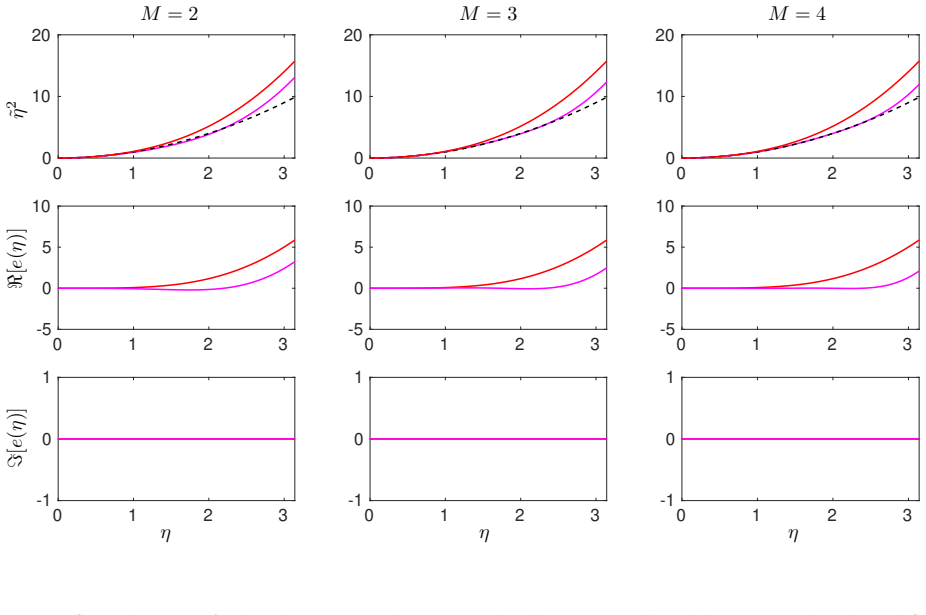
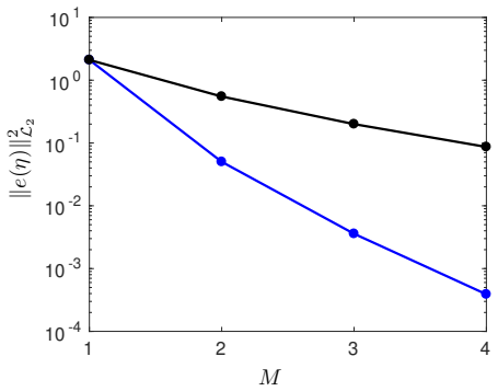
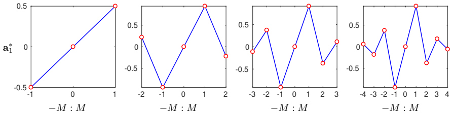
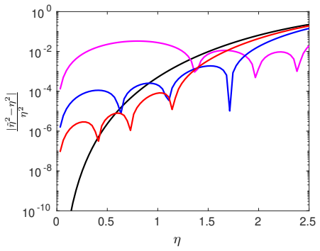
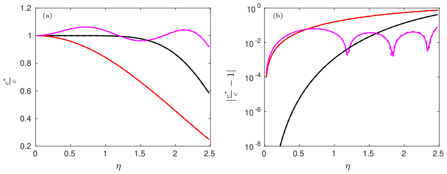
On its own terms, the paper establishes that the optimal finite-difference coefficients for a derivative of order $d$ and a given stencil are the solution of the quadratic program in Eq. (52): minimize the weighted $L^2$ norm of the spectral error $e(\eta)=\sum_m a_m e^{jm\eta}-(j\eta)^d$ subject to order-accuracy constraints and, when full discretization is considered, a linear-matrix-inequality stability constraint obtained by bounding the 2-norm of the evolution operator. For the accuracy-plus-spectral problem, the KKT equations give the coefficients in closed form, and the paper proves two structural results: for even $d$ the optimal error is purely real, so the coefficients are symmetric, and for odd $d$ it is purely imaginary, so the coefficients are antisymmetric. When stability is added, the framework yields schemes that bias only the odd-derivative stencils—upwinding the convective term—while leaving even-derivative stencils symmetric, and it can produce explicit schemes whose guaranteed stable time steps are about an order of magnitude larger than those of standard schemes of the same order. The paper also shows numerically that optimized second-order schemes can reproduce the physics of diffusion, advection-diffusion, Burgers, and wave problems with accuracy comparable to or better than standard eighth-order schemes, especially at high wavenumbers.
Load-bearing premise
The load-bearing premise is that bounding the 2-norm of the evolution operator by one is a faithful enough proxy for true spectral-radius stability; if that bound is much looser than the actual stability limit for non-normal operators, then the very-large-time-steps result is a guaranteed lower bound rather than an exact characterization.
Editorial extensions
If this is right
- Spectral resolution and formal order of accuracy cease to be tied: with a fixed stencil and low formal order, optimized schemes can resolve high wavenumbers far better than standard high-order schemes of the same stencil.
- Stability-aware optimization produces upwinded first-derivative stencils and symmetric second-derivative stencils, giving a principled justification for the common practice of stabilizing convection while leaving diffusion central.
- Explicit schemes can be designed to remain stable at time steps an order of magnitude larger than standard explicit schemes by accepting larger spectral error, which is directly useful for massively parallel simulations where implicit time stepping is costly.
- Existing optimized schemes, such as dispersion-relation-preserving and low-dissipation low-dispersion explicit schemes, are recovered by the framework as special cases, so the framework unifies them rather than competing with them.
- Semi-discrete stability of the optimized schemes depends only on the even-derivative terms of the PDE, so stability can be assessed and enforced term by term.
Reading between the lines
- Beyond the paper: the same optimization with a non-constant $\gamma(\eta)$ could be used to design schemes that preserve a target dispersion relation over a prescribed band, effectively turning Eq. (52) into a dispersion-relation-preserving design tool with built-in stability.
- Beyond the paper: since the 2-norm stability condition is sufficient but not necessary, replacing it with the exact spectral-radius condition or a pseudospectral bound would likely enlarge the guaranteed stable region in Figs. 8 and 9; this is a testable numerical extension using eigenvalue computations.
- Beyond the paper: the framework's symmetry and antisymmetry proofs rely only on the form of the spectral error and the positivity of $\gamma$, so they should carry over to boundary stencils and to compact (implicit) finite differences, provided the stencil is expressed in the same linear form.
- Beyond the paper: a natural next step, which the authors flag as ongoing, is to optimize space and time discretizations jointly; the current framework fixes the temporal scheme and would need a non-convex treatment to couple both.
Signed reviews
Editorial analysis
A structured set of objections, weighed in public.
Referee Report
Summary. The paper proposes a unified optimization framework for deriving finite-difference schemes that simultaneously accounts for formal order of accuracy, spectral resolution, and stability. Order conditions are written as linear equality constraints, spectral error is minimized as a weighted L2 norm in wavenumber space, and stability of the fully discrete scheme is imposed through a matrix 2-norm bound expressed as a linear matrix inequality. For the accuracy-plus-spectral subproblem, the authors derive an analytical KKT solution and prove that the optimal stencil is symmetric for even derivatives and antisymmetric for odd derivatives, yielding purely dissipative or purely dispersive spectral errors, respectively. Stability is then treated either by maximizing the time step for a fixed optimal stencil or by optimizing stencil coefficients for a fixed time step under the stability constraint. The framework is applied to diffusion, linear advection-diffusion, Burgers, and wave equations, with comparisons against standard finite differences and analytical solutions. The central claim is that the most general formulation, Eq. (52), is a well-posed convex problem whose solutions expose exploitable tradeoffs between accuracy and stability, including explicit schemes stable at very large time steps.
Significance. If the claims hold, this is a valuable contribution to computational physics: it provides a mathematically clean, problem-specific way to design finite-difference operators, and it unifies strands of the optimized-scheme literature (e.g., dispersion-relation-preserving and bandwidth-optimized schemes) under one convex formulation. The analytical KKT solution and the symmetry/antisymmetry lemmas are genuine structural results, and the numerical tests against analytical solutions of the diffusion, advection-diffusion, and Burgers equations provide credible support for the performance claims. The paper also correctly identifies and demonstrates an interesting tradeoff: for fixed formal order, additional stencil points can be spent on stability rather than on spectral accuracy, with the odd-derivative stencil absorbing the bias. The main reservations are a gap in the justification that the stability-constrained problem reduces to O(Sd) degrees of freedom, and a mathematical misstatement in the stability condition as written.
major comments (2)
- [Sec. 2.3.4, Eq. (52); Lemma 3] The assertion that 'as a consequence of Lemma 3 for periodic domains, the optimization problem in Eq. (52) has a total of n = Sd degrees of freedom' is not justified by Lemma 3 as stated and proved. Appendix C proves uniformity of the optimal stencil only for the equality-constrained quadratic program (46)-(48), whose KKT system does not include the stability LMI (45). Since the objective and the stability constraint in Eq. (52) are invariant under cyclic permutation of the grid-point rows, one can in fact recover a uniform-row minimizer by averaging over cyclic shifts, but this argument is not given. Please either supply this missing argument or reformulate Eq. (52) directly over a single stencil and state that the periodic stability analysis is performed on the resulting circulant operator. Without this, the claimed O(Sd) computational cost and the interpretation of Figs. 9-11 are not fully supported.
- [Sec. 2.3.2, Eq. (43)] The stability condition is written as lambda_max(I_N + sum_d (Delta t/(Delta x)^d) beta_d A_d^Phi) <= 1. For the non-symmetric evolution operator in Eq. (42), in particular for the advective (skew-symmetric) part, eigenvalues need not be real, so 'lambda_max' is not defined and this inequality is neither necessary nor sufficient for the spectral-radius condition needed for bounded powers of the evolution operator. The subsequent replacement by the 2-norm bound in Eq. (44) is correct and is what the numerical results actually use, but Eq. (43) should be corrected to rho(...) <= 1, with the usual caveat about semisimple unit-modulus eigenvalues.
minor comments (6)
- [Appendices A and B, Sec. 4] The proofs of Lemmas 1 and 2 conclude that the antisymmetric (or symmetric) part vanishes from integral conditions involving S^T a or C^T a. This conclusion requires gamma to be positive, or at least supported on a set of positive measure where the finite trigonometric sums are linearly independent. The examples with gamma = 0 outside [0, 2.5] satisfy this, but the statement in Section 4 that symmetry holds 'regardless of the functional form of gamma(eta)' is too broad as written; the required hypothesis on gamma should be stated in the lemmas.
- [Sec. 2.3.2, Eq. (44)] The paper should state explicitly that for the periodic uniform grids used in Figs. 8-10 the evolution operator is circulant and hence normal, so ||G||_2 = rho(G) and the 2-norm LMI is not conservative for those cases. This would clarify why the stability regions are tight, and it would underline the caveat, already given for multistep schemes in Sec. 2.3.5, that the 2-norm bound can be conservative for the non-periodic extension sketched in Sec. 4.
- [Sec. 3.2] The text near Fig. 14 refers to 'SDF2' and 'SDF8'; these should be 'SFD2' and 'SFD8' for consistency with the rest of the paper.
- [Sec. 3.2] The statement that the framework reproduces the schemes of [3,8] is made only qualitatively. A short table or error comparison would give readers a concrete way to verify that claim.
- [Throughout] There are numerous typographical errors and inconsistencies (e.g., 'exmaple', 'dicrete', 'dissiption', 'meangingful', 'stems for' instead of 'stems from'). A careful proofreading pass is needed before publication.
- [Sec. 3] No code or data repository is provided. Since the paper's central tool is a convex optimization formulation solved with cvx, releasing the scripts and full coefficient tables would materially improve reproducibility and would allow readers to test the stability-region claims independently.
Circularity Check
No circularity found: the optimization framework is self-contained and its derived properties follow from the stated minimization and constraints.
full rationale
The paper's central claim is that Eq. (52) minimizes a weighted L2 spectral error, defined independently in Eq. (19) as the difference between the modified and exact wavenumber responses, subject to the order-accuracy equalities Eq. (30) and the stability LMI Eq. (45). The coefficients are not fitted to any target output; the KKT solution Eq. (25) follows from positive definiteness of Qd and full row rank of Xd, and Lemmas 1 and 2 are proven in Appendices A and B by decomposing stencils into symmetric and antisymmetric parts. The stability regions in Figs. 8-10 are generated from the LMI condition, not from matching a desired stability boundary, and the numerical tests in Sec. 3 compare against analytical solutions (Eqs. 62, 64, 67) rather than against the optimization objective. The only backward-looking validation, the statement in Sec. 3.2 that optimized fourth-order schemes reproduce the coefficients of Refs. [3,8], is an external check, not an input to the derivation. No self-citation is load-bearing, and no fitted parameter is renamed as a prediction. The acknowledged conservativeness of the 2-norm bound in Sec. 2.3.5 is a limitation, not a circularity.
Assumptions & free parameters
assumptions (5)
- standard math Fourier/modal analysis defines spectral error via modified wavenumber (Section 2.2).
- standard math Karush-Kuhn-Tucker conditions solve the equality-constrained quadratic program (Eq. 24).
- standard math Schur complement equivalence for the LMI in Eq. (45).
- domain assumption Uniform grid and periodic domain for all analytical results (Section 2.3.4 and Appendix D).
- domain assumption The matrix 2-norm bound is a sufficient proxy for spectral-radius stability (Eq. 44).
Cite this review
Pith. "Pith review of A Unified Approach for Deriving Optimal Finite Differences." pith.science (2026). https://pith.science/paper/AL4OPSU7
@misc{pith2026190802890,
  author       = {Pith},
  title        = {Pith review of: A Unified Approach for Deriving Optimal Finite Differences},
  year         = {2026},
  howpublished = {\url{https://pith.science/paper/AL4OPSU7}},
  note         = {Machine review of arXiv:1908.02890}
}
read the original abstract
A unified approach to derive optimal finite differences is presented which combines three critical elements for numerical performance especially for multi-scale physical problems, namely, order of accuracy, spectral resolution and stability. The resulting mathematical framework reduces to a minimization problem subjected to equality and inequality constraints. We show that the framework can provide analytical results for optimal schemes and their numerical performance including, for example, the type of errors that appear for spectrally optimal schemes. By coupling the problem in this unified framework, one can effectively decouple the requirements for order of accuracy and spectral resolution, for example. Alternatively, we show how the framework exposes the tradeoffs between e.g. accuracy and stability and how this can be used to construct explicit schemes that remain stable with very large time steps. We also show how spectrally optimal schemes only bias odd-order derivatives to remain stable, at the expense of accuracy, while leaving even-order derivatives with symmetric coefficients. Schemes constructed within this framework are tested for diverse model problems with an emphasis on reproducing the physics accurately.
Figures

Figures from the paper (16 more)







Reference graph
Works this paper leans on
-
[1]
Hirsch, Numerical computation of internal and external flows, volume 1, Wiley, New York, 1994
C. Hirsch, Numerical computation of internal and external flows, volume 1, Wiley, New York, 1994
work page 1994
-
[2]
S. K. Lele, Compact finite-difference schemes with spectral-like resolution, J. Comp. Phys. 103 (1992) 16–42
work page 1992
-
[3]
C. K. Tam, J. C. Webb, Dispersion-relation-preserving finite difference schemes for computational acoustics, J. Comp. Phys. 107 (1993) 262 – 281
work page 1993
-
[4]
J. W. Kim, D. J. Lee, Optimized compact finite difference schemes with maximum resolution, AIAA Journal 34 (1996) 887–893
work page 1996
-
[5]
Z. Wang, R. Chen, Optimized weighted essentially nonoscillatory schemes for linear waves with discon- tinuity, J. Comp. Phys. 174 (2001) 381 – 404
work page 2001
- [6]
-
[7]
D. Ponziani, S. Pirozzoli, F. Grasso, Development of optimized weighted-ENO schemes for multiscale compressible flows, Int. J. Numer. Meth. Fluids 42 (2003) 953–977
work page 2003
- [8]
Show all 25 references
-
[9]
M. P. Martin, E. M. Taylor, M. Wu, V. G. Weirs, A bandwidth-optimized WENO scheme for the effective direct numerical simulation of compressible turbulence, J. Comp. Phys. 220 (2006) 270–289
2006
-
[10]
T. K. Sengupta, S. K. Sircar, A. Dipankar, High accuracy schemes for DNS and acoustics, Journal of Scientific Computing 26 (2006) 151–193
2006
-
[11]
J. Fang, Z. Li, L. Lu, An optimized low-dissipation monotonicity-preserving scheme for numerical simulations of high-speed turbulent flows, J. Sci. Comput. 56 (2013) 67–95
2013
-
[12]
Zhang, Z.-X
J.-H. Zhang, Z.-X. Yao, Optimized explicit finite-difference schemes for spatial derivatives using maxi- mum norm, J. Comp. Phys. 250 (2013) 511 – 526
2013
-
[13]
Pirozzoli, Performance analysis and optimization of finite-difference schemes for wave propagation problems, J
S. Pirozzoli, Performance analysis and optimization of finite-difference schemes for wave propagation problems, J. Comp. Phy. 222 (2007) 809–831
2007
-
[14]
Ashcroft, X
G. Ashcroft, X. Zhang, Optimized prefactored compact schemes, J. Comp. Phys. 190 (2003) 459 – 477
2003
-
[15]
Haras, S
Z. Haras, S. Ta’asan, Finite difference schemes for long-time integration, J. Comp. Phy. 114 (1994) 265 – 279
1994
-
[16]
Sengupta, G
T. Sengupta, G. Ganeriwal, S. De, Analysis of central and upwind compact schemes, J. Comp. Phy. 192 (2003) 677 – 694
2003
-
[17]
T. K. Sengupta, A. Bhole, Error dynamics of diffusion equation: Effects of numerical diffusion and dispersive diffusion, Journal of Computational Physics 266 (2014) 240 – 251
2014
-
[18]
D. P. Bertsekas, Nonlinear programming, Athena scientific Belmont, 1999
1999
-
[19]
Grant, S
M. Grant, S. Boyd, Y. Ye, CVX: Matlab software for disciplined convex programming, 2008
2008
-
[20]
Ben-Tal, A
A. Ben-Tal, A. Nemirovski, Lectures on modern convex optimization: analysis, algorithms, and engi- neering applications, SIAM, 2001. 34
2001
-
[21]
Stoer, R
J. Stoer, R. Bulirsch, Introduction to numerical analysis, volume 12, Springer Science & Business Media, 2013
2013
-
[22]
R. Y. Zhang, J. Lavaei, Efficient algorithm for large-and-sparse LMI feasibility problems, IEEE CDC (2018) 6868–6875
2018
-
[23]
Eberhard, The partial differential equation ut +uux =µuxx, Communications on Pure and Applied Mathematics 3 (1950) 201–230
H. Eberhard, The partial differential equation ut +uux =µuxx, Communications on Pure and Applied Mathematics 3 (1950) 201–230
1950
-
[24]
J. D. Cole, On a quasi-linear parabolic equation occurring in aerodynamics, Quarterly of Applied Mathematics 9 (1951) 225–236
1951
-
[25]
Shokin, K
Y. Shokin, K. Roesner, The Method of Differential Approximation, Scientific Computation, Springer Berlin Heidelberg, 2011. 35
2011
Reviewed August 14, 2026 · model on record in the stance chip above.
Discussion (0). Continue with ORCID to comment.