REVIEW 3 major objections 6 minor 6 references
Viterbi Extraction tutorial with Hidden Markov Toolkit
T0 review · 3 major / 6 minor · reviewed 2026-08-14 · deepseek-v4-flash
Pith's one-line read This paper works through HTK's HInit Viterbi extraction by hand: recurrence equations, traceback matrix, and a full parameter update.
desk verdict A standard-algorithm tutorial whose worked numbers disagree with its own equations; the outline is sound but the example is not reproducible. read the letter →
The pith
A machine-rendered reading of the paper's core claim, the machinery that carries it, and where it could break.
The reading
What carries the argument
The machinery is the Viterbi recursion with log-Gaussian emission costs and a backtrack matrix. The forward equation $\delta_t(j)=\max_i[\delta_{t-1}(i)a_{ij}]b_j(O_t)$ fills a cost grid with the best log-probability of reaching each state at each time, while the companion equation $\psi_t(j)=\arg\max_i[\delta_{t-1}(i)a_{ij}]$ records the predecessor state that achieved it. The termination and backtracking equations (5) through (7) turn those tables into a single best state sequence. The paper makes the mechanism concrete by printing the $\delta$ values inside the circles of figures 4 and 5 and the predecessor choices in TABLE III.
What would settle it
Recompute equation (3) for t=2 using the printed transition matrix (13), the Gaussian parameters in TABLE II, and observation $\mathbf{x}_2$ from TABLE I, with $\delta_1(2)=-4.1817$. A direct evaluation gives $\delta_2(2)\approx -8.1996$ rather than the printed $-7.1013$; checking the remaining delta entries against the same formulas would show whether the worked example faithfully executes the algorithm.
Extended reading notes
Core claim
The central claim is that the algorithm implemented in HTK's HInit is exactly the Baum-Viterbi estimation procedure, and that its operation can be captured by equations (2) through (7): $\delta_1(j)=\pi_j b_j(O_1)$, $\delta_t(j)=\max_i[\delta_{t-1}(i)a_{ij}]b_j(O_t)$, $\psi_t(j)=\arg\max_i[\delta_{t-1}(i)a_{ij}]$, termination by $P^*=\max_i \delta_T(i)$, and backtracking $q_t^*=\psi_{t+1}(q_{t+1}^*)$. The 12-observation, 4-state illustration is the demonstration: TABLE I gives the observations, TABLE II seeds the Gaussian parameters by uniform segmentation, TABLE III records the traceback matrix, TABLE IV lists the extracted best path 1, 2, 2, 3, 2, 2, 2, 3, 2, 3, 2, 3, 3, 4, and TABLE V updates the Gaussian parameters for the next iteration. The paper claims convergence by the criterion $|P_k^* - P_{k-1}^*| \le \epsilon$, shown in TABLE VI, reaching $-18.87455$ by iteration five.
Load-bearing premise
The demonstration rests on the printed numbers actually coming from the printed formulas and inputs; if a shown cost value cannot be reproduced from the transition matrix, Gaussian parameters, and observations, the worked example does not show the algorithm working.
Editorial extensions
If this is right
- Equations (2) through (7) are sufficient to re-implement HInit-style Viterbi training in any programming language.
- Uniform segmentation works as a seed for Viterbi training when no prior state alignment exists.
- The best-state path from the backtrack matrix yields direct re-estimates of both the transition matrix and the Gaussian means and variances.
- The stopping rule compares best-path log scores across iterations; with threshold 0.0001, the example converges at iteration 5.
Reading between the lines
- Given the paper's transparency goal, a companion script that regenerates figures 4 and 5 from the printed inputs would make the tutorial self-checking; the t=2 arithmetic in the printed example suggests readers should verify before reusing the tables.
- The same recurrence loop would extend to Gaussian-mixture observation densities by summing over mixture components in the emission term and re-estimating mixture weights during the update; the single-Gaussian choice is a simplification, not a limit of the method.
- Once the parameters are estimated, the very same delta and psi tables can be used to decode new observation sequences; the paper frames them as training artifacts, leaving the decoding use implicit.
Signed reviews
Editorial analysis
A structured set of objections, weighed in public.
Referee Report
Summary. This paper is a tutorial on the Viterbi extraction (segmental k-means / hard EM) algorithm for HMM parameter estimation as implemented in HTK's HInit. It reviews the standard recurrence equations (2)-(7), defines a four-state HMM with two emitting states, and presents a 12-observation example. The example includes uniform segmentation initialization (Table II), per-time delta values and backtracking (Figs. 4-5, Table III), the extracted state sequence (Table IV), parameter updates (Table V and the transition matrix in (15)), and a convergence table (Table VI). The paper explicitly disclaims any performance claim and states that the purpose is purely expository.
Significance. If the numerical example were internally consistent, this would be a useful pedagogical resource: it addresses a real gap, the concrete numerical behavior of HInit, and it is transparent about its scope. The paper's strength is its explicit walk-through with figures and tables, and it makes no overreaching accuracy claims. However, the printed deltas in Section III-E do not reproduce from the stated formulas and inputs, and the equations are ambiguous between probability-domain and log-domain quantities. Because the tutorial's value depends on readers being able to verify the calculation, these issues are central rather than cosmetic. The paper does not present machine-checked proofs or code; its contribution is expository.
major comments (3)
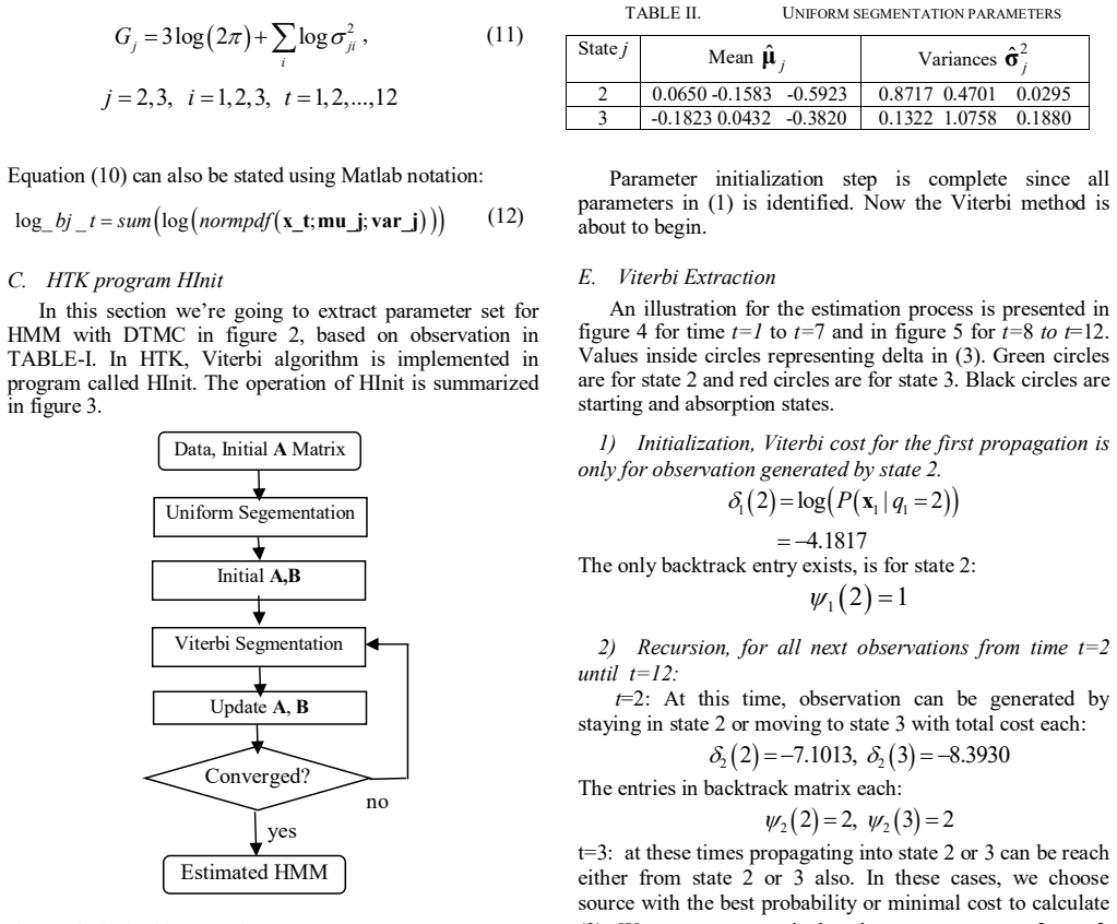
- [Section III-E, Eq. (3), Eq. (13), Table II] The printed Viterbi deltas for t=2 do not follow from the stated inputs. Using Eq. (3) with δ1(2)=−4.1817, the initial transition matrix (13), and the Gaussian parameters in Table II for observation t=2 of Table I, I obtain δ2(2)≈−8.1996 and δ2(3)≈−8.9560, in agreement with Fig. 4. The text instead reports δ2(2)=−7.1013 and δ2(3)=−8.3930. Since Section III-E is the paper's only worked demonstration that Eqs. (2)-(7) describe HInit, these discrepancies must be corrected; a reader cannot verify the algorithm from the printed values. The figures and Table VI appear to use the corrected values, so the error is likely localized to the prose, but it is nevertheless load-bearing.
- [Section II-B, Eqs. (2)-(7), Section III-E] The paper never states whether the recurrence is carried out in the probability domain or the log domain. Equations (2)-(3) multiply probabilities and b_j(O_t), but every numerical value in Section III-E is a log cost (e.g., −4.1817, −7.1013, and the termination in Eq. (14) adds log a34), and the text refers to 'total cost' and 'minimum cost.' A reader implementing directly from (3) would obtain different numbers. The tutorial should explicitly define δ_t(j) and ψ_t(i) as log-domain quantities and write the log-domain recursions, e.g., δ_t(j) = max_i [δ_{t−1}(i)+log a_ij] + log b_j(O_t), before presenting the example.
- [Section III-B, Eqs. (10)-(11)] The Gaussian log-likelihood formula is not typeset correctly: the quadratic term appears to divide by σ_ji rather than σ_ji^2, and the normalization term is split between (10) and (11) in a way that is ambiguous (the factor 1/2 and the constant G are not clearly attached). Since all delta values and parameter updates depend on this formula, the paper should give a single, unambiguous expression for log b_j(O_t) and ensure it is the one used to produce Tables II-VI.
minor comments (6)
- [Section III-F, Eq. (15)] Equation (15) is numbered twice: once for the updated transition matrix and once for the convergence criterion. Please renumber the second occurrence and update the cross-reference 'based on (15)'.
- [Section III-E, t=3 values] The printed values for δ3(2) and δ3(3) are hard to read ('10.59' and '10. 2 81'); please ensure the minus signs and spacing are typeset cleanly.
- [TABLE III] The header row 'state' and the row labels 2,3,4 are confusing; please clarify that the first row gives the time index and the row labels are the candidate states.
- [References] Reference [5] is incomplete ('Acoustics, Speech and Signal …') and should be expanded to the full publication title.
- [Abstract] The sentence 'This writing merely to describe how the algorithm is performed' is ungrammatical; please rephrase it.
- [Eq. (9)] The notation [b_2(t) b_3(t)] for B is unclear; please define the vector/matrix indexing explicitly.
Circularity Check
No significant circularity: the paper is a self-contained tutorial that describes, rather than claims to derive, the Viterbi extraction algorithm.
full rationale
The paper does not present a derived prediction or a first-principles result; its stated purpose is explicitly tutorial: 'This writing merely to describe how the algorithm is performed.' The Viterbi recurrences in equations (2)-(7) are standard textbook equations cited to Rabiner [2] and the HTK Book [1], not results claimed to be newly derived here. The numerical example in Section III is an illustration of those recurrences, and the manually updated transition and Gaussian parameters in (15) and TABLE V are computed from the segmentation produced by the same recurrences, which is the normal operation of an iterative estimation algorithm rather than a fitted input being renamed as a prediction. The references are to external standard sources (Rabiner, HTK, Juang and Rabiner, Caliebe and Rösler), not to prior work by the same authors, so no self-citation chain is load-bearing. The abstract and Section IV contain honest limitations: the paper does not justify performance or accuracy and notes that more massive and varying data would be needed for further explanation. A separate numerical-consistency concern exists: the printed delta values in Section III-E, such as delta_2(2) = -7.1013, do not appear to follow from the stated formulas and Table II inputs, while the figure values appear consistent with recomputation. That is an internal-consistency or correctness defect in the exposition, not a circularity: the example depends transparently on its inputs, and the paper makes no claim that the printed deltas were independently predicted. There is no step in which an output quantity is equivalent by construction to an input quantity, no parameter fitted to a subset of data then presented as a prediction of a closely related quantity, and no uniqueness theorem imported from the authors' own prior work. The finding is therefore no significant circularity, score 0.
Assumptions & free parameters
free parameters (3)
- Initial transition matrix A
- Uniform segmentation boundary =
6 observations per state
- Convergence threshold epsilon =
0.0001
assumptions (4)
- standard math HMM is defined by parameter set (A, B, pi) as in equation (1).
- domain assumption Observation vectors are generated by independent Gaussian distributions for each component.
- domain assumption HTK's HInit implements the described Viterbi training procedure.
- standard math The Viterbi recurrence (3) with backtracking (7) yields the most likely state sequence.
Cite this review
Pith. "Pith review of Viterbi Extraction tutorial with Hidden Markov Toolkit." pith.science (2026). https://pith.science/paper/QQBGVUAE
@misc{pith2026190803143,
  author       = {Pith},
  title        = {Pith review of: Viterbi Extraction tutorial with Hidden Markov Toolkit},
  year         = {2026},
  howpublished = {\url{https://pith.science/paper/QQBGVUAE}},
  note         = {Machine review of arXiv:1908.03143}
}
read the original abstract
An algorithm used to extract HMM parameters is revisited. Most parts of the extraction process are taken from implemented Hidden Markov Toolkit (HTK) program under name HInit. The algorithm itself shows a few variations compared to another domain of implementations. The HMM model is introduced briefly based on the theory of Discrete Time Markov Chain. We schematically outline the Viterbi method implemented in HTK. Iterative definition of the method which is ready to be implemented in computer programs is reviewed. We also illustrate the method calculation precisely using manual calculation and extensive graphical illustration. The distribution of observation probability used is simply independent Gaussians r.v.s. The purpose of the content is not to justify the performance or accuracy of the method applied in a specific area. This writing merely to describe how the algorithm is performed. The whole content should enlighten the audience the insight of the Viterbi Extraction method used by HTK.
Figures


Figures from the paper (1 more)

Reference graph
Works this paper leans on
-
[1]
The HTK Book version 3.5 alpha,
S. Young, E. Gunnar, G. Mark, T. Hain, and D. K ershaw, “The HTK Book version 3.5 alpha,” Cambridge University, 2015
work page 2015
-
[2]
A Tutorial on Hidden Markov Mod els and Selected Applications in Speech Recognition,
L. R. Rabiner, “A Tutorial on Hidden Markov Mod els and Selected Applications in Speech Recognition,” in Proceedings of the IEEE , 1989, vol. 77, no. 2, pp. 257–286
work page 1989
-
[3]
Osaki, Applied Stochastic System Modeling
S. Osaki, Applied Stochastic System Modeling . 2002
work page 2002
-
[4]
S. B. Davis and P. Mermelstein, “Comparison of Parametric Representations for Monosyllabic Word Recognition i n Continuously Spoken Sentences,” IEEE Trans. Acoust. , vol. 28, no. 4, pp. 357–366, 1980
work page 1980
-
[5]
The segmental K -means algorithm for estimating parameters of hidden Markov models,
B. H. Juang and L. R. Rabiner, “The segmental K -means algorithm for estimating parameters of hidden Markov models,” Acoustics, Speech and Signal … , vol. 38, no. 9. pp. 1639–1641, 1990
work page 1990
-
[6]
Convergence of the M aximum A Posteriori Path Estimator in Hidden Markov Models,
A. Caliebe and U. Rösler, “Convergence of the M aximum A Posteriori Path Estimator in Hidden Markov Models,” IEEE Trans. Inf. Theory , vol. 48, no. 7, pp. 1750–1758, 2002. Zulkarnaen Hatala was born in Ambon, on 19 Agustus 1977. He received Sarjana Teknik on Informatics at 2002 and Master Teknik on Telecommunications at 2005. Both degress are from Telkom ...
work page 2002
Reviewed August 14, 2026 · model on record in the stance chip above.
Discussion (0). Continue with ORCID to comment.