REVIEW 3 major objections 4 minor 30 references
WhiteNNer-Blind Image Denoising via Noise Whiteness Priors
T0 review · 3 major / 4 minor · reviewed 2026-08-14 · deepseek-v4-flash
Pith's one-line read A convolutional network can separate signal from noise in a single noisy image without ground truth, using noise whiteness priors, and this blind approach beats established self-supervised and classical denoisers on confocal endomicroscopy.
desk verdict Useful blind-denoising idea with an honest ablation, but the 'decoupling without ground truth' claim outruns the loss design and the synthetic-only evaluation. read the letter →
The pith
A machine-rendered reading of the paper's core claim, the machinery that carries it, and where it could break.
The reading
What carries the argument
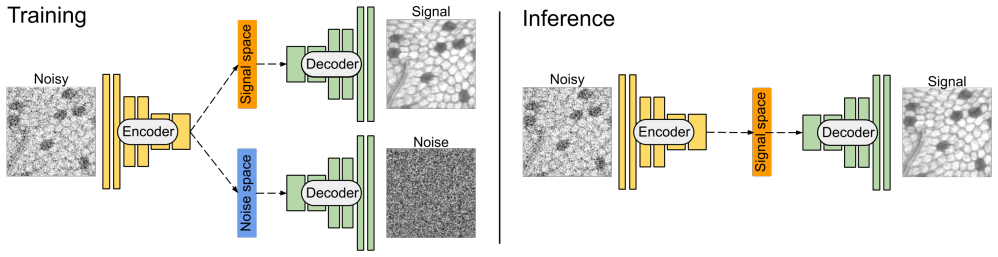
The load-bearing mechanism is the two-tailed latent-space separation combined with a four-term loss. The network is a U-Net whose encoder produces two separate latent representations, $F_S$ and $F_N$, decoded by a shared decoder; at inference only $F_S$ is kept. The loss is $L_{rec} + L_{pc} + L_{tv} + L_{ac} + L_{st}$, where $L_{rec}$ enforces $S+N=X$, $L_{pc}$ and $L_{tv}$ encode signal smoothness, $L_{ac}$ minimizes sample auto-correlation of the noise at nonzero lags, and $L_{st}$ penalizes spatial variance imbalance across blocks. Together these priors are intended to single out the true decomposition from the continuum of possible splits.
What would settle it
Acquire noisy CLE frames together with clean references obtained by averaging many registered frames; run WhiteNNer and check whether its denoised output matches the averaged reference better than Noise2Self, and whether the estimated noise is measurably white—if the noise estimate shows significant autocorrelation at nonzero lags or if the reconstruction is no better than the reference when noise is realistic, the central claim is refuted.
Extended reading notes
Core claim
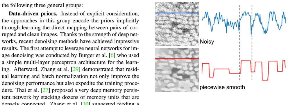
The paper's central claim is that blind denoising can be solved by treating the noisy input as the sum of a signal and a noise field, and training a two-branch encoder–decoder (dubbed WhiteNNer) to output both components simultaneously. One branch produces the latent code for the signal, the other for the noise; a shared decoder reconstructs both in the spatial domain, and the reconstruction loss enforces $S + N = X$. The signal is regularized by total variation and a piecewise-constancy loss computed from a graph-based segmentation of the input; the noise is regularized by an auto-correlation loss that penalizes non-zero correlation at nonzero lags and a stationarity loss that forces equal variance across image blocks. The authors state that this design makes their network the first able to decouple signal and noise without ground truth, and report higher PSNR and SSIM than Noise2Self, NLM and BM3D on three CLE datasets at $\sigma=50$, with the gap widening at higher noise levels.
Load-bearing premise
The load-bearing premise is that the image degradation is additive white Gaussian noise and that the four hand-crafted priors are strong enough to pick the true signal out of the infinitely many ways to split a noisy image into signal plus noise.
Editorial extensions
If this is right
- Blind denoising becomes possible from a single noisy image: no clean reference, no paired noisy frames, and no input noise-level parameter are required.
- The explicit two-branch design beats the single-output variant, so forcing the network to represent noise separately in latent space is itself a useful regularizer.
- Each loss term contributes: removing any prior lowers PSNR, with the auto-correlation whiteness term alone adding 2.74 dB on CLE100 at $\sigma=50$.
- Across $\sigma \in \{15, 25, 35, 50, 75\}$, WhiteNNer-2 stays ahead of Noise2Self on CLE100, and its advantage over blind baselines grows as noise increases.
Reading between the lines
- The same whiteness-prior recipe might transfer to other imaging modalities (e.g., fluorescence microscopy, ultrasound) whose noise is approximately white, giving a plug-in replacement for supervised denoisers.
- Because the network outputs an actual noise field, one could test whether the estimated noise is truly white; if it is, the method could double as a noise-model validator for a given sensor.
- The method is only validated on synthetic AWGN; if real CLE noise is correlated or non-stationary, the priors may bias the decomposition, so an obvious extension is evaluating on real noisy frames with ground truth from frame averaging.
Signed reviews
Editorial analysis
A structured set of objections, weighed in public.
Referee Report
Summary. The paper proposes WhiteNNer, a U-Net-based blind denoising method for confocal laser endomicroscopy (CLE) images that outputs both a signal estimate and a noise estimate from a single noisy input. Training is self-supervised in the sense that no ground-truth clean images are used; the loss combines a reconstruction term enforcing S+N=X, total variation and piecewise-constancy priors on the signal, and auto-correlation and stationarity priors on the noise. Experiments on three public CLE datasets with synthetic additive white Gaussian noise (AWGN) report PSNR/SSIM improvements over NLM, BM3D, Noise2Self, and near-parity with Noise2Noise/Noise2True, along with an ablation study and paired t-tests. The paper claims to be the first model capable of decoupling signal and noise without ground truth.
Significance. If the results hold, the paper offers a practical self-supervised denoising approach for medical imaging where clean references are unavailable. The two-branch architecture that explicitly separates signal and noise at the output is a simple and potentially transferable idea, and the joint use of signal and noise whiteness priors is a reasonable contribution. Strengths include held-out evaluation with five-model error bars, an ablation showing that each loss term contributes to PSNR, and statistical significance testing against several baselines. However, the evaluation is restricted to synthetic AWGN, and the 'blind' claim is stronger than the loss design supports; the revision should either add experiments that substantiate true blind generalization across noise levels or temper the claim.
major comments (3)
- [3.2] Equations (5), (8), and (10)-(11) define noise priors that do not constrain the variance of the predicted noise. Lac only penalizes non-zero-lag autocorrelation, which is zero for any white noise regardless of its amplitude, and Lst is minimized whenever the block standard deviations are equal, independent of their common value. Consequently, the only term that determines how much of X is assigned to N is the TV prior (Eq. 13) with a hand-set coefficient of 5e-5. This makes the decomposition S+N=X non-identifiable unless the noise level is known from the training distribution. The paper does not demonstrate that a single trained model generalizes across noise levels: Figure 5 reports performance at various sigma, but the text does not state whether separate models are trained for each sigma. If separate models are used, the 'blind' claim in the title and abstract is not supported. The authors should either add a noise-level anchor to the loss, evaluate one model at multiple sigma values, or substantially qualify the blind-denosing claim.
- [4.1] All experiments are performed on real CLE images corrupted with synthetic AWGN, which is exactly the noise model assumed in Eq. (1). The claimed practical value for CLE imaging is therefore not tested against actual acquisition noise, which may be correlated or non-stationary. I request an experiment on real noisy CLE data (e.g., pairs or repeated frames) or at least a discussion of how the whiteness priors would behave under realistic noise. Without this, the central application claim remains unvalidated.
- [5] The conclusion states that 'our network is the first model that is capable of decoupling the signal and noise components without ground truth information.' This is too strong: Noise2Self also produces a signal estimate whose residual is a noise estimate and requires no ground truth. The novelty of WhiteNNer is better positioned as the explicit two-branch output and the joint use of signal and noise priors, rather than decoupling per se. Please revise the claim to avoid an unsubstantiated priority assertion.
minor comments (4)
- [3.2] Equation (9) defines the sample autocorrelation with a scalar lag in [1, M], while Eq. (7) uses 2D lags (l,m). Please specify how the random lag is sampled for 2D images and how the padded image is used to compute the sample autocorrelation.
- [4.2] Figure 5: clarify whether each CNN-based method is retrained for each sigma level or whether a single model is applied across levels; this is essential for interpreting the 'blind' claim.
- [4.3] Table 4: the ablation trains each configuration for 100 epochs, while the main results use 500 epochs. Please state whether the relative ordering of loss terms is stable at 500 epochs or provide the full-training ablation.
- [2] In Related Works, 'Tsai tet al.' should read 'Tsai et al.'
Circularity Check
No significant circularity: the loss terms are independently defined priors, results are benchmarked on held-out CLE splits, and no fitted parameter is renamed as a prediction.
full rationale
The paper's derivation chain is an empirical objective, not a first-principles derivation that reduces to its own inputs. The total loss in Eq. (2) is an explicit sum of reconstruction fidelity and independently motivated priors: autocorrelation loss (Eq. 8), stationarity loss (Eq. 11), piecewise-constancy loss (Eq. 12), and TV loss (Eq. 13). None of these terms is defined in terms of the final PSNR/SSIM targets, and no parameter is fitted to a subset of the evaluation data and then renamed as a prediction. There are no self-citations to prior work by the same authors, and no uniqueness theorem is imported. The method is trained on synthetically corrupted images and evaluated on held-out test splits of three public CLE datasets, so the reported improvements over NLM, BM3D, Noise2Self, and Noise2Noise are external benchmark evidence rather than a tautology of the loss. The strongest caveat is that the signal/noise split is not identifiable from the loss alone: the whiteness terms are scale-free, and the hand-set TV coefficient (5e-5) controls how much energy is pushed into the noise output. That is an identifiability and generalization concern about the claimed blind-decoupling capability, not a circular derivation. Per the review rules, concerns about overclaiming or untested real-noise assumptions belong to correctness risk, not circularity. Therefore no circular step is established.
Assumptions & free parameters
free parameters (3)
- TV loss weight =
5e-5
- Stationary loss block sizes =
b randomly chosen from {2, 4, 8, 16} per update
- Felzenszwalb-Huttenlocher segmentation parameters for Lpc
assumptions (4)
- domain assumption Noise is additive white Gaussian with fixed sigma.
- domain assumption Noise is ergodic and the image is large enough that sample auto-correlation approximates the ensemble auto-correlation.
- domain assumption The signal is piecewise constant with low total variation, and graph segmentation of the noisy image provides a valid piecewise-constant target.
- ad hoc to paper The combined loss uniquely and adequately separates S from N despite infinitely many decompositions satisfying S+N=X.
Cite this review
Pith. "Pith review of WhiteNNer-Blind Image Denoising via Noise Whiteness Priors." pith.science (2026). https://pith.science/paper/E3MTF672
@misc{pith2026190803238,
  author       = {Pith},
  title        = {Pith review of: WhiteNNer-Blind Image Denoising via Noise Whiteness Priors},
  year         = {2026},
  howpublished = {\url{https://pith.science/paper/E3MTF672}},
  note         = {Machine review of arXiv:1908.03238}
}
read the original abstract
The accuracy of medical imaging-based diagnostics is directly impacted by the quality of the collected images. A passive approach to improve image quality is one that lags behind improvements in imaging hardware, awaiting better sensor technology of acquisition devices. An alternative, active strategy is to utilize prior knowledge of the imaging system to directly post-process and improve the acquired images. Traditionally, priors about the image properties are taken into account to restrict the solution space. However, few techniques exploit the prior about the noise properties. In this paper, we propose a neural network-based model for disentangling the signal and noise components of an input noisy image, without the need for any ground truth training data. We design a unified loss function that encodes priors about signal as well as noise estimate in the form of regularization terms. Specifically, by using total variation and piecewise constancy priors along with noise whiteness priors such as auto-correlation and stationary losses, our network learns to decouple an input noisy image into the underlying signal and noise components. We compare our proposed method to Noise2Noise and Noise2Self, as well as non-local mean and BM3D, on three public confocal laser endomicroscopy datasets. Experimental results demonstrate the superiority of our network compared to state-of-the-art in terms of PSNR and SSIM.
Figures

Figures from the paper (2 more)


Reference graph
Works this paper leans on
-
[1]
M. S. C. Almeida and M. A. T. Figueiredo. Parameter es- timation for blind and non-blind deblurring using residual whiteness measures. IEEE Transactions on Image Process- ing, 22(7):2751–2763, 2013. 3
work page 2013
-
[2]
J. Batson and L. Royer. Noise2Self: Blind denoising by self- supervision. In International Conference on Machine Learn- ing, volume 97, pages 524–533, 2019. 2, 6, 7
work page 2019
-
[3]
F. Bray, J. Ferlay, I. Soerjomataram, R. L. Siegel, L. A. Torre, and A. Jemal. Global cancer statistics 2018: GLOBOCAN estimates of incidence and mortality worldwide for 36 can- cers in 185 countries. CA: a cancer journal for clinicians , 68(6):394–424, 2018. 1
work page 2018
- [4]
- [5]
-
[6]
H. C. Burger, C. J. Schuler, and S. Harmeling. Image de- noising: Can plain neural networks compete with BM3D? In IEEE Conference on Computer Vision and Pattern Recogni- tion, pages 2392–2399, 2012. 3
work page 2012
- [7]
-
[8]
W. Dong, L. Zhang, G. Shi, and X. Li. Nonlocally central- ized sparse representation for image restoration.IEEE Trans- actions on Image Processing, 22(4):1620–1630, 2013. 2
work page 2013
Show all 30 references
-
[9]
Elad and M
M. Elad and M. Aharon. Image denoising via sparse and redundant representations over learned dictionaries. IEEE Transactions on Image Processing, 15(12):3736–3745,
-
[10]
P. F. Felzenszwalb and D. P. Huttenlocher. Efficient graph- based image segmentation. International Journal of Com- puter Vision, 59(2):167–181, 2004. 5
2004
-
[11]
Grisan, E
E. Grisan, E. Veronese, G. Diamantis, C. Trovato, C. Crosta, and G. Battaglia. Computer aided diagnosis of Barrett’s esophagus using confocal laser endomicroscopy: Prelimi- nary data. Gastrointestinal Endoscopy, 75(4,):AB126, 2012. 5
2012
-
[12]
S. Guo, Z. Yan, K. Zhang, W. Zuo, and L. Zhang. Toward convolutional blind denoising of real photographs. In IEEE Conference on Computer Vision and Pattern Recognition ,
-
[13]
P. C. Hansen, M. E. Kilmer, and R. H. Kjeldsen. Exploiting residual information in the parameter choice for discrete ill- posed problems. BIT Numerical Mathematics, 46(1):41–59,
-
[14]
Kiesslich, J
R. Kiesslich, J. Burg, M. Vieth, J. Gnaendiger, M. Enders, P. Delaney, A. Polglase, W. McLaren, D. Janell, S. Thomas, and B. Nafe. Confocal laser endoscopy for diagnosing in- traepithelial neoplasias and colorectal cancer in vivo. Gas- troenterology, 127:706–713, 2004. 2
2004
-
[15]
Kiesslich, L
R. Kiesslich, L. Gossner, M. Goetz, A. Dahlmann, M. Vi- eth, M. Stolte, A. Hoffman, M. Jung, B. Nafe, P. Galle, and M. Neurath. In vivo histology of Barretts esophagus and as- sociated neoplasia by confocal laser endomicroscopy. Clini- cal Gastroenterology and Hepatology, 4(8)...
2006
-
[16]
Lanza, S
A. Lanza, S. Morigi, F. Sgallari, and A. J. Yezzi. Variational image denoising based on autocorrelation whiteness. SIAM Journal on Imaging Sciences, 6(4):1931–1955, 2013. 3
1931
-
[17]
Lehtinen, J
J. Lehtinen, J. Munkberg, J. Hasselgren, S. Laine, T. Kar- ras, M. Aittala, and T. Aila. Noise2Noise: Learning image restoration without clean data. In International Conference on Machine Learning, volume 80, pages 2965–2974, 2018. 2, 6
2018
-
[18]
Lempitsky, A
V . Lempitsky, A. Vedaldi, and D. Ulyanov. Deep image prior. In IEEE Conference on Computer Vision and Pattern Recognition, pages 9446–9454, 2018. 3
2018
-
[19]
R. W. Leong, N. Q. Nguyen, C. Meredith, S. AlSohaily, D. Kukic, P. M. Delaney, E. R. Murr, J. Yong, N. D. Merrett, and A. V . Biankin. In vivo confocal endomicroscopy in the diagnosis and evaluation of celiac disease.Gastroenterology, 135(6):1870 – 1876, 2008. 5
2008
-
[20]
X. Liu, M. Tanaka, and M. Okutomi. Single-image noise level estimation for blind denoising. IEEE Transactions on Image Processing, 22(12):5226–5237, 2013. 7
2013
-
[21]
Mumford and J
D. Mumford and J. Shah. Optimal approximations by piecewise smooth functions and associated variational prob- lems. Communications on pure and applied mathematics , 42(5):577–685, 1989. 3, 4, 5
1989
-
[22]
Ronneberger, P
O. Ronneberger, P. Fischer, and T. Brox. U-Net: Convolu- tional networks for biomedical image segmentation. InMed- ical Image Computing and Computer-Assisted Intervention , pages 234–241, 2015. 3, 4
2015
-
[23]
L. I. Rudin, S. Osher, and E. Fatemi. Nonlinear total varia- tion based noise removal algorithms. Physica D: Nonlinear Phenomena, 60(1):259 – 268, 1992. 2, 3, 4, 5
1992
-
[24]
B. W. Rust and D. P. O’Leary. Residual periodograms for choosing regularization parameters for ill-posed problems. Inverse Problems, 24(3):034005, 2008. 3
2008
-
[25]
Soltanayev and S
S. Soltanayev and S. Y . Chun. Training deep learning based denoisers without ground truth data. In Advances in Neural Information Processing Systems 31, pages 3257–3267. 2018. 3
2018
-
[26]
Stefanescu, C
D. Stefanescu, C. Streba, E. T. Cartana, A. Saftoiu, G. Gruionu, and L. G. Gruionu. Computer aided diagno- sis for confocal laser endomicroscopy in advanced colorectal adenocarcinoma. PloS ONE, 11(5):e0154863, 2016. 5
2016
-
[27]
Y . Tai, J. Yang, X. Liu, and C. Xu. MemNet: A persis- tent memory network for image restoration. In IEEE Inter- national Conference on Computer Vision, pages 4549–4557,
-
[28]
A. Tsai, A. Yezzi, and A. S. Willsky. Curve evolution implementation of the Mumford-Shah functional for image segmentation, denoising, interpolation, and magnification. IEEE Transactions on Image Processing, 10(8):1169–1186,
-
[29]
Zhang, W
K. Zhang, W. Zuo, Y . Chen, D. Meng, and L. Zhang. Be- yond a Gaussian denoiser: Residual learning of deep CNN for image denoising. IEEE Transactions on Image Process- ing, 26(7):3142–3155, 2017. 2, 3
2017
-
[30]
Zhang, W
K. Zhang, W. Zuo, and L. Zhang. FFDNet: Toward a fast and flexible solution for CNN-based image denoising. IEEE Transactions on Image Processing, 27(9):4608–4622, 2018. 2, 3
2018
Reviewed August 14, 2026 · model on record in the stance chip above.
Discussion (0). Continue with ORCID to comment.