Trajectory-wise Control Variates for Variance Reduction in Policy Gradient Methods

Byron Boots; Ching-An Cheng; Xinyan Yan

REVIEW 3 major objections 4 minor 46 references

Trajectory-wise Control Variates for Variance Reduction in Policy Gradient Methods

T0 review · 3 major / 4 minor · reviewed 2026-08-14 · deepseek-v4-flash

Challenge this review Re-run · record.json Download PDF Read on arXiv ↗ Review JSON

Pith's one-line read The paper claims that the natural chronological ordering of states and actions yields the optimal trajectory-wise control variate for policy gradients, cutting variance from future policy randomness at no extra learning cost.

desk verdict The TrajCV estimator is sound and the variance decomposition is useful, but the paper's headline optimality result rests on a proof step that goes beyond Lemma A.1's independence assumption. read the letter →

arxiv 1908.03263 v1 pith:UFS4R5JT submitted 2019-08-08 cs.LG stat.ML

Ching-An Cheng , Xinyan Yan , Byron Boots This is my paper · ORCID

classification cs.LGstat.ML

keywords policygradientcontrolvariatesvariancereductionreinforcementlearningtrajectory-wiseQ-functionlawoftotalMonteCarloestimation

verification ladder T0 review T1 audit T2 compute T3 formal

The pith

A machine-rendered reading of the paper's core claim, the machinery that carries it, and where it could break.

The reading

Policy gradient estimates suffer from high variance because the Monte Carlo gradient of one time step is correlated with random future states and actions. This paper argues that existing state-only and state-action control variates miss that trajectory structure, and it proposes trajectory-wise control variates (TrajCV) that subtract, for every future step, the policy-dependent part of the future return. The construction is recursive, needs only a Q-function approximator (the same object existing methods learn), and remains unbiased. Under the paper's assumptions the proposed estimator is optimal among all orderings of the random variables used to decompose the variance, reducing variance substantially when dynamics are nearly deterministic. A reader should care because variance is the main driver of sample inefficiency in policy-gradient reinforcement learning.

What carries the argument

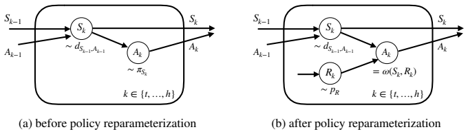
The load-bearing object is the difference estimator built from a recursive law-of-total-variance decomposition. For each gradient component $G_t$, the paper orders the random variables causally, identifies the variance attributed to each future action $A_k$, and chooses the optimal CV for that term, which is a function of $(S_k,A_k)$ whose conditional expectation over $A_k$ is available because only the policy distribution is used. Summing these per-step terms gives estimator (12); the optimality proof rests on an inequality (Lemma A.1) saying that conditioning on an earlier variable leaves no more residue, plus a feasibility argument based on the Bayes network that blocks unknown-dynamics dependencies when action randomness precedes future states. The natural ordering is what makes the CV computable from the Q-function alone.

What would settle it

Enumerate all feasible orderings on a small three-step MDP with known dynamics, a Gaussian policy, and an exact Q-function, and compute the residue variance remaining after each ordering's optimal CV; if any feasible ordering has strictly smaller residue than the natural ordering, Theorem 4.1 is false.

Watch

Extended reading notes

Core claim

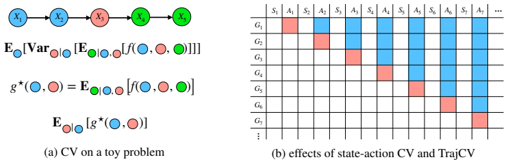
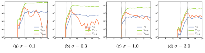
The paper's central claim is that the natural chronological ordering $S_t\to A_t\to S_{t+1}\to A_{t+1}\to\cdots\to S_h\to A_h$ is the best ordering for designing a control variate for each policy gradient component $G_t=N_t C_{t:h}$, and that the estimator (12) is the optimal trajectory-wise control variate in the sense of minimizing the residue variance once the optimal CV for each ordering is attainable. The estimator subtracts from $G_t$ the sum over $k$ from $t$ to $h$ of $\left(N_t \hat{Q}_k - \mathbb{E}_{A_k|S_k}[N_t \hat{Q}_k]\right)$, which cancels variance caused by policy randomness at every future action while leaving the expectation unchanged. With deterministic dynamics and an exact Q-function, all of the variance $V_{A_t|S_t}$ and $V_{|S_t,A_t}$ is removed from each component. The paper also shows by a variance decomposition that the third term $V_{|S_t,A_t}$, ignored by previous state-action CVs, is as large as the action-conditional term for Gaussian policies with small variance, which is why the extra terms matter.

Load-bearing premise

The optimality theorem depends on an inequality that is proven only for independent variables being applied to dependent MDP variables during the ordering exchanges in the proof; if that step fails, the natural ordering may not be optimal, though the estimator would still be unbiased.

Editorial extensions

If this is right

Long horizons become less punishing: the dominant long-term variance $V_{|S_t,A_t}$ is reduced by the extra terms, whereas state-action CVs leave it untouched.
Sample efficiency improves without changing the learning target: only a Q-function approximator is required, the same object as existing state-action control variates.
When transition dynamics are deterministic and the Q-function estimate is accurate, the per-component variance collapses to only the state-marginal term $V_{S_t}$.
Trajectory-wise CVs can be computed in $O(h)$ time per trajectory, so the variance gain does not require additional rollouts.

Reading between the lines

Editorial extensions of the paper, not claims the author makes directly.

The paper's optimality argument assumes exact Q-functions; in practice, with imperfect critics, a different ordering that samples action randomness first could beat the natural ordering when a learned dynamics model is more accurate than the Q-function estimate.
The same divide-and-conquer variance decomposition should carry over to off-policy or importance-weighted policy gradients, where the known distribution is the behavior policy rather than the target policy; that is a testable extension the paper does not develop.
Viewing state-action baselines as the diagonal of an upper-triangular variance structure suggests a general recipe: any known conditional distribution along a trajectory can supply an unbiased per-step control variate.

Share X Bluesky LinkedIn Reddit HN

Signed reviews

No signed human review yet.

Editorial analysis

A structured set of objections, weighed in public.

Desk editor's note, referee report, and a circularity audit.

Desk Editor's Note

read the letter

The paper is worth a serious look. The core idea—augmenting state-action control variates with additional Q-function terms along the trajectory—is simple and sensible, and the derivation via the divide-and-conquer law-of-total-variance argument is genuinely new, even if the resulting estimator (12) was already in Pankov's technical report, which the authors honestly acknowledge. The variance component analysis (Theorem 3.1) and the ordering-optimality claim (Theorem 4.1) are the real novelties, and they are presented clearly enough to engage with directly.

What the paper does well: the unbiasedness of TrajCV is immediate from the control-variate construction, and the recursive computation using only Q-function approximators is practical. The self-contained theory has no fitted constants, and the citations are appropriate. The empirical section is honest but preliminary—one deterministic CartPole domain, approximate critics, no code—so it mainly serves as a sanity check rather than a demonstration of the method's power in complex continuous control.

The soft spot is Theorem 4.1. The proof in Appendix A.1 relies on Lemma A.1, which is proven only for independent X and Y, but the exchange operations move dependent MDP variables (e.g., Rk and Su) without verifying the required conditional independence structure. The stress-test note is right: operation (b) appears to assume that moving Rk after Su does not increase residue, but the lemma's hypothesis is not met in the Bayes net where Rk is an ancestor of Su. Also, the claimed feasibility condition for operation (b) looks internally inconsistent with the definition of feasible orderings. This is a real gap in the proof of the paper's headline optimality claim.

However, this gap does not sink the paper. The estimator (12) remains unbiased regardless of Theorem 4.1, and the variance decomposition in (13) is plausible and useful on its own. The optimality claim is important but not load-bearing for the practical method—it is a theoretical bonus that should be either fixed or softened to a conjecture. The authors seem aware that the proof is sketchy ("proof is deferred to Appendix A" without much detail), so I suspect it can be repaired, but as written it is not established.

For peer review: yes, a serious referee should engage with this. The paper deserves revision rather than rejection. The reviewer should push for a complete proof of Theorem 4.1 or a clear statement of the additional assumptions needed. I would cite the estimator and the variance analysis in my own work, and I would bring it to a reading group focused on policy gradient theory, though the current proof gap tempers enthusiasm.

Referee Report

3 major / 4 minor

Summary. The paper studies control variates for policy-gradient estimation in finite-horizon MDPs. It observes that the usual state-action control variate (6) reduces only the variance due to the action at the current step, and proposes TrajCV, which adds terms for later steps so that the estimator (12) also reduces variance due to future policy randomness along the trajectory. The construction is derived by repeatedly applying the law of total variance under the ordering (11), and the authors claim in Theorem 4.1 that this natural ordering minimizes the residual variance among all orderings of the reparameterized variables when the optimal control variate for each ordering is attainable. Section 3 gives asymptotic variance bounds for Gaussian policies (Theorem 3.1), and Section 5 reports CartPole experiments comparing naive Monte Carlo, state-dependent CV, state-action CV, and TrajCV.

Significance. If Theorem 4.1 were established, the paper would give a clean optimality justification for a simple and practical variance-reduction scheme that requires only approximate Q-functions and can be computed recursively. The estimator itself is unbiased, and the divide-and-conquer derivation in Section 4.1 is transparent and useful. Theorem 3.1 also provides a concrete asymptotic picture of why the future-trajectory variance component matters. However, the proof of Theorem 4.1 in Appendix A.1 relies on an unproved extension of Lemma A.1 to dependent variables, and the reduction to the natural ordering is not rigorously established; the headline optimality claim is therefore not currently supported by the manuscript.

major comments (3)

[Appendix A.1, Lemma A.1 and operation (b)] Lemma A.1 proves inequality (15) only for independent X and Y. Operation (b) moves R_k after S_u in the reparameterized Bayes net of Figure 2b, where R_k is an ancestor of S_u and the two variables are dependent. The proof asserts that this exchange does not increase the residue 'because of the discussion after Lemma A.1', but no conditional-independence or d-separation conditions are verified at this step. Without such a generalized inequality, the optimality of the natural ordering in Theorem 4.1 is unproven; for dependent variables the inequality in Lemma A.1 can fail. This is load-bearing for the paper's central claim.
[Appendix A.1, operation (b)] The configuration S_v -> R_k -> S_u with v > u > k is incompatible with the proof's own definition of a feasible ordering, which requires R_k to appear before S_{k+1,h}. If S_v appears before R_k and v > u > k, then a state after k appears before R_k, violating feasibility. Thus the exchange operation described in the proof cannot be applied to any feasible ordering, and the claimed transformation to the natural ordering is not well-defined. A different exchange argument or a formal characterization of feasible orderings is needed.
[Appendix A.1, operation (a)] The statement that two states S_v and S_u with v > u can be exchanged 'without affecting residue' is asserted without computation. States in the MDP are dependent through the dynamics, and the residue is defined through conditional expectations and variances with respect to a specific ordering; changing the order of states changes the conditioning sets in the law-of-total-variance decomposition. This invariance requires proof, not assertion, and this gap is independent of the issue with dependent action randomness.

minor comments (4)

[Section 4.2, Eq. (12)] The displayed estimator has summation indices ∑_{t=1}^h and then ∑_{k=1}^h; for component G_t the sum should be over k = t, ..., h. As written the first sum is ill-defined and inconsistent with the preceding display. Please correct the indices.
[Figures 4 and 5] The legend entries such as 'state-action CV (MC)' and 'TrajCV (MC)' are not self-explanatory; the caption should state that MC refers to the 1000-sample approximation of E_{A|S}[\hat Q].
[Notation, Eqs. (7)-(8) and Figure 3] The third variance component is written V_{|S_t,A_t} in Eq. (8) but V_{|A_t,S_t} in Figure 3; please use one consistent ordering of the subscripts.
[Introduction, related work] The text acknowledges that reference [24] reports exactly equation (12), but the relation is only discussed in the final paragraph of the introduction; it would be clearer to state this overlap explicitly when the estimator is introduced.

Circularity Check

0 steps flagged · score 0.0 of 10

No circularity found: the trajectory-wise control variate derivation is self-contained, with no fitted parameter renamed as a prediction and no load-bearing self-citation.

full rationale

The paper's central claim is that the estimator (12) is an optimal trajectory-wise control variate and that the natural ordering (11) minimizes residue variance. The derivation constructs the estimator from a recursive law-of-total-variance decomposition, with the Q-function approximator as a standard learned input rather than a parameter fitted to force the result. Theorem 4.1 is proved in Appendix A.1 using Lemma A.1 and ordering-exchange operations; the theorem's conclusion is not assumed by any definition. The possible weakness identified in the proof, namely that Lemma A.1 is stated for independent X and Y while the exchange operation moves dependent MDP variables, is a rigor or correctness gap, not circularity: it does not reduce the theorem to its statement. The paper's self-citations ([6] and [8]) appear in citation clusters for convergence guarantees and policy optimization speed, and they are not used to justify the main variance-reduction result or to forbid alternative orderings. The experimental section compares against standard Monte Carlo and existing control-variate baselines, so no fitted input is relabeled as a prediction. Therefore the derivation chain is self-contained and no circular step can be exhibited.

Assumptions & free parameters 0 free parameters · 7 assumptions · 0 invented entities

The theory is parameter-free; all randomness is modeled by the stated MDP and policy. The only ad hoc objects are the optimal-CV attainability assumption and the unproved separation/exchange properties used in the optimality proof.

assumptions (7)

standard math Law of total variance with nested conditioning
Used in Eq (7), (10), and (13) to decompose variance into per-step components.
standard math Jensen's inequality in Lemma A.1 for independent X and Y
Proves Var_X E_Y[f] <= E_Y Var_X[f], the basis for ordering comparisons.
domain assumption MDP with finite horizon, known cost, unknown dynamics and policy
Problem setup in Section 2; all results assume this model.
domain assumption Gaussian policy, bounded cost, Q-function analytic in action, small sigma for Theorem 3.1
Stated in Theorem 3.1; used to derive the O(h^2/sigma^4) variance scaling.
ad hoc to paper Optimal CV of a given ordering is attainable (exact Q-function)
Theorem 4.1 assumes this; in practice Q-function approximators are imperfect, so the optimality result is conditional.
ad hoc to paper Fact 1 separation property: a CV term affects only its corresponding variance component
Stated as a fact with a toy illustration but not formally proved for the MDP setting; essential for summing CVs in Eq (12).
ad hoc to paper Generalized exchange inequality for dependent MDP variables (extension of Lemma A.1)
Operation (b) in Appendix A.1 moves R_k after S_u claiming no increase in residue; the conditional-independence conditions are not verified.

how reviews work

0 comments

Cite this review

Pith. "Pith review of Trajectory-wise Control Variates for Variance Reduction in Policy Gradient Methods." pith.science (2026). https://pith.science/paper/UFS4R5JT

@misc{pith2026190803263,
  author       = {Pith},
  title        = {Pith review of: Trajectory-wise Control Variates for Variance Reduction in Policy Gradient Methods},
  year         = {2026},
  howpublished = {\url{https://pith.science/paper/UFS4R5JT}},
  note         = {Machine review of arXiv:1908.03263}
}

read the original abstract

Policy gradient methods have demonstrated success in reinforcement learning tasks that have high-dimensional continuous state and action spaces. However, policy gradient methods are also notoriously sample inefficient. This can be attributed, at least in part, to the high variance in estimating the gradient of the task objective with Monte Carlo methods. Previous research has endeavored to contend with this problem by studying control variates (CVs) that can reduce the variance of estimates without introducing bias, including the early use of baselines, state dependent CVs, and the more recent state-action dependent CVs. In this work, we analyze the properties and drawbacks of previous CV techniques and, surprisingly, we find that these works have overlooked an important fact that Monte Carlo gradient estimates are generated by trajectories of states and actions. We show that ignoring the correlation across the trajectories can result in suboptimal variance reduction, and we propose a simple fix: a class of "trajectory-wise" CVs, that can further drive down the variance. We show that constructing trajectory-wise CVs can be done recursively and requires only learning state-action value functions like the previous CVs for policy gradient. We further prove that the proposed trajectory-wise CVs are optimal for variance reduction under reasonable assumptions.

Figures

Figures reproduced from arXiv: 1908.03263 by the authors.

**Figure 2.** Bayes networks for the random variables in [PITH_FULL_IMAGE:figures/full_fig_p007_2.png] view at source ↗

**Figure 3.** The size of components of Tr (Var[Gt]) during training, for t = 100, evaluated at policies generated under the “upper bound” setting that emulates noiseless estimates for the CartPole problem with horizon h = 1000. Different initial values for σ of the Gaussian policy (defined in Theorem 3.1) are used. The x axis denotes the iteration, and the y axis is in log scale. The two vertical dashed lines mark the boundaries… view at source ↗

Discussion (0). Continue with ORCID to comment.

Reference graph

Works this paper leans on

46 extracted references · 39 canonical work pages

[1]

R. J. Williams. Simple statistical gradient-following algorithms for connectionist reinforce- ment learning. Machine learning, 8(3-4):229–256, 1992

work page 1992
[2]

R. S. Sutton, D. A. McAllester, S. P. Singh, and Y . Mansour. Policy gradient methods for reinforcement learning with function approximation. In Advances in Neural Information Pro- cessing Systems, pages 1057–1063, 2000

work page 2000
[3]

S. M. Kakade. A natural policy gradient. In Advances in Neural Information Processing Systems, pages 1531–1538, 2002

work page 2002
[4]

Peters and S

J. Peters and S. Schaal. Natural actor-critic. Neurocomputing, 71(7-9):1180–1190, 2008

work page 2008
[5]

Schulman, S

J. Schulman, S. Levine, P. Abbeel, M. Jordan, and P. Moritz. Trust region policy optimization. In International Conference on Machine Learning, pages 1889–1897, 2015

2015
[6]

Cheng, X

C.-A. Cheng, X. Yan, N. Ratliff, and B. Boots. Predictor-corrector policy optimization. In International Conference on Machine Learning, 2019

work page 2019
[7]

V . R. Konda and J. N. Tsitsiklis. Actor-critic algorithms. In Advances in Neural Information Processing Systems, pages 1008–1014, 2000

work page 2000
[8]

Cheng, X

C.-A. Cheng, X. Yan, N. Wagener, and B. Boots. Fast policy learning through imitation and reinforcement. In Conference on Uncertainty in Artiﬁcial Intelligence, 2018

work page 2018

Show all 46 references

[9]

Yang and Y

L. Yang and Y . Zhang. Policy optimization with stochastic mirror descent. arXiv preprint arXiv:1906.10462, 2019

1906 arXiv
[10]

Ghadimi, G

S. Ghadimi, G. Lan, and H. Zhang. Mini-batch stochastic approximation methods for non- convex stochastic composite optimization. Mathematical Programming, 155(1-2):267–305, 2016

2016
[11]

Kimura, S

H. Kimura, S. Kobayashi, et al. An analysis of actor-critic algorithms using eligibility traces: reinforcement learning with imperfect value functions. Journal of Japanese Society for Artiﬁ- cial Intelligence, 15(2):267–275, 2000

2000
[12]

P. Thomas. Bias in natural actor-critic algorithms. In International Conference on Machine Learning, pages 441–448, 2014

2014
[13]

Silver, G

D. Silver, G. Lever, N. Heess, T. Degris, D. Wierstra, and M. Riedmiller. Deterministic policy gradient algorithms. In International Conference on Machine Learning, 2014

2014
[14]

Schulman, P

J. Schulman, P. Moritz, S. Levine, M. Jordan, and P. Abbeel. High-dimensional continuous control using generalized advantage estimation. In International Conference on Learning Rep- resentations, 2016

2016
[15]

W. Sun, J. A. Bagnell, and B. Boots. Truncated horizon policy search: Combining reinforce- ment learning & imitation learning. In International Conference on Learning Representations, 2018

2018
[16]

Efroni, G

Y . Efroni, G. Dalal, B. Scherrer, and S. Mannor. Beyond the one step greedy approach in reinforcement learning. In International Conference on Machine Learning, 2019

2019
[17]

A. Y . Ng, D. Harada, and S. Russell. Policy invariance under reward transformations: The- ory and application to reward shaping. In International Conference on Machine Learning , volume 99, pages 278–287, 1999

1999
[18]

Greensmith, P

E. Greensmith, P. L. Bartlett, and J. Baxter. Variance reduction techniques for gradient esti- mates in reinforcement learning. Journal of Machine Learning Research, 5(Nov):1471–1530, 2004

2004
[19]

Jie and P

T. Jie and P. Abbeel. On a connection between importance sampling and the likelihood ratio policy gradient. In Advances in Neural Information Processing Systems , pages 1000–1008, 2010. 11

2010
[20]

S. Gu, T. Lillicrap, Z. Ghahramani, R. E. Turner, and S. Levine. Q-prop: Sample-efﬁcient policy gradient with an off-policy critic. In International Conference on Learning Representa- tions, 2017

2017
[21]

H. Liu, Y . Feng, Y . Mao, D. Zhou, J. Peng, and Q. Liu. Action-depedent control variates for policy optimization via stein’s identity. In International Conference on Learning Representa- tions, 2018

2018
[22]

Grathwohl, D

W. Grathwohl, D. Choi, Y . Wu, G. Roeder, and D. Duvenaud. Backpropagation through the void: Optimizing control variates for black-box gradient estimation. In International Confer- ence on Learning Representations, 2018

2018
[23]

Tucker, S

G. Tucker, S. Bhupatiraju, S. Gu, R. E. Turner, Z. Ghahramani, and S. Levine. The mirage of action-dependent baselines in reinforcement learning. arXiv preprint arXiv:1802.10031, 2018

2018 arXiv
[24]

S. Pankov. Reward-estimation variance elimination in sequential decision processes. arXiv preprint arXiv:1811.06225, 2018

2018 arXiv
[25]

C. Wu, A. Rajeswaran, Y . Duan, V . Kumar, A. M. Bayen, S. Kakade, I. Mordatch, and P. Abbeel. Variance reduction for policy gradient with action-dependent factorized baselines. In International Conference on Learning Representation, 2018

2018
[26]

R. Bellman. A Markovian decision process. Journal of Mathematics and Mechanics , pages 679–684, 1957

1957
[27]

D. P. Bertsekas, D. P. Bertsekas, D. P. Bertsekas, and D. P. Bertsekas. Dynamic programming and optimal control, volume 1. Athena scientiﬁc Belmont, MA, 1995

1995
[28]

Beck and M

A. Beck and M. Teboulle. Mirror descent and nonlinear projected subgradient methods for convex optimization. Operations Research Letters, 31(3):167–175, 2003

2003
[29]

S. M. Kakade et al. On the sample complexity of reinforcement learning. PhD thesis, University of London London, England, 2003

2003
[30]

Vemula, W

A. Vemula, W. Sun, and J. A. Bagnell. Contrasting exploration in parameter and action space: A zeroth-order optimization perspective. In International Conference on Artiﬁcial Intelligence and Statistics, 2019

2019
[31]

S. M. Ross. A course in simulation. Prentice Hall PTR, 1990

1990
[32]

A. B. Owen. Monte Carlo theory, methods and examples. 2013

2013
[33]

Schmidt, N

M. Schmidt, N. Le Roux, and F. Bach. Minimizing ﬁnite sums with the stochastic average gradient. Mathematical Programming, 162(1-2):83–112, 2017

2017
[34]

Johnson and T

R. Johnson and T. Zhang. Accelerating stochastic gradient descent using predictive variance reduction. In Advances in Neural Information Processing Systems, pages 315–323, 2013

2013
[35]

Defazio, F

A. Defazio, F. Bach, and S. Lacoste-Julien. Saga: A fast incremental gradient method with support for non-strongly convex composite objectives. In Advances in Neural Information Processing Systems, pages 1646–1654, 2014

2014
[36]

C. Wang, X. Chen, A. J. Smola, and E. P. Xing. Variance reduction for stochastic gradient optimization. In Advances in Neural Information Processing Systems, pages 181–189, 2013

2013
[37]

Ciosek and S

K. Ciosek and S. Whiteson. Expected policy gradients for reinforcement learning. arXiv preprint arXiv:1801.03326, 2018

2018 arXiv
[38]

S. P. Singh and R. S. Sutton. Reinforcement learning with replacing eligibility traces. Machine learning, 22(1-3):123–158, 1996

1996
[39]

K. L. Chung. A course in probability theory. Academic press, 2001

2001
[40]

Baxter and P

J. Baxter and P. L. Bartlett. Inﬁnite-horizon policy-gradient estimation. Journal of Artiﬁcial Intelligence Research, 15:319–350, 2001. 12

2001
[41]

Landau and E

L. Landau and E. Lifshitz. Statistical physics (course of theoretical physics vol 5). 1958

1958
[42]

Brockman, V

G. Brockman, V . Cheung, L. Pettersson, J. Schneider, J. Schulman, J. Tang, and W. Zaremba. OpenAI Gym. arXiv preprint arXiv:1606.01540, 2016

2016 arXiv
[43]

J. Lee, M. X. Grey, S. Ha, T. Kunz, S. Jain, Y . Ye, S. S. Srinivasa, M. Stilman, and C. K. Liu. DART: Dynamic animation and robotics toolkit. The Journal of Open Source Software, 3(22): 500, feb 2018

2018
[44]

C. M. Bishop. Pattern recognition and machine learning. springer, 2006. 13 Appendix A Missing Proofs A.1 Proof for Theorem 4.1 To understand how the ordering matters, we consider a toy example of estimating EX,Y [f(X,Y )] of some functionf of two random variablesX andY . We pr...

2006
[45]

That is, a feasible ordering must be causal at least in actions: the action randomness that causes a state must be arranged before that state in the ordering

We show that when dynamics is the MDP is unknown, an ordering is feasible, if and only if,Rk appears beforeSk+1,h for allt≤k <h. That is, a feasible ordering must be causal at least in actions: the action randomness that causes a state must be arranged before that state in the...
[46]

We consider the following operations (a) Suppose, in an ordering, there isSv→Su,v >u, then we can exchange them without affecting residue

We show that any feasible ordering can be transformed into the natural ordering in (11) using operations that do not increase the residue. We consider the following operations (a) Suppose, in an ordering, there isSv→Su,v >u, then we can exchange them without affecting residue....

Pith tools

Reviewed August 14, 2026 · model on record in the stance chip above.

[1] [1]

R. J. Williams. Simple statistical gradient-following algorithms for connectionist reinforce- ment learning. Machine learning, 8(3-4):229–256, 1992

work page 1992

[2] [2]

R. S. Sutton, D. A. McAllester, S. P. Singh, and Y . Mansour. Policy gradient methods for reinforcement learning with function approximation. In Advances in Neural Information Pro- cessing Systems, pages 1057–1063, 2000

work page 2000

[3] [3]

S. M. Kakade. A natural policy gradient. In Advances in Neural Information Processing Systems, pages 1531–1538, 2002

work page 2002

[4] [4]

Peters and S

J. Peters and S. Schaal. Natural actor-critic. Neurocomputing, 71(7-9):1180–1190, 2008

work page 2008

[5] [5]

Schulman, S

J. Schulman, S. Levine, P. Abbeel, M. Jordan, and P. Moritz. Trust region policy optimization. In International Conference on Machine Learning, pages 1889–1897, 2015

2015

[6] [6]

Cheng, X

C.-A. Cheng, X. Yan, N. Ratliff, and B. Boots. Predictor-corrector policy optimization. In International Conference on Machine Learning, 2019

work page 2019

[7] [7]

V . R. Konda and J. N. Tsitsiklis. Actor-critic algorithms. In Advances in Neural Information Processing Systems, pages 1008–1014, 2000

work page 2000

[8] [8]

Cheng, X

C.-A. Cheng, X. Yan, N. Wagener, and B. Boots. Fast policy learning through imitation and reinforcement. In Conference on Uncertainty in Artiﬁcial Intelligence, 2018

work page 2018