REVIEW 3 major objections 4 minor 50 references
Applying the matched-filter technique to the search for dark matter transients with networks of quantum sensors
T0 review · 3 major / 4 minor · reviewed 2026-08-14 · deepseek-v4-flash
Pith's one-line read A matched-filter search over GPS atomic clock data can detect thin domain-wall dark matter transients at 95 percent probability for clock jumps as small as 0.045 nanoseconds.
desk verdict A solid method paper that derives the right analytic SNR for common-reference clock networks and demonstrates it in simulation, but the promised calibrated archival search depends on noise assumptions not yet tested on real GPS data. read the letter →
The pith
A machine-rendered reading of the paper's core claim, the machinery that carries it, and where it could break.
The reading
What carries the argument
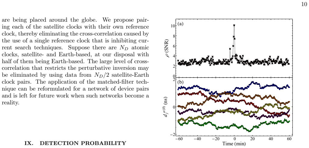
The carrying mechanism is the matched-filter SNR built from the inverse network covariance matrix. Each trial signal is a thin-domain-wall template (Eq. 22): in the differenced clock stream it is a single spike of height $h_a$ at the epoch the wall hits a satellite clock, and a spike of opposite sign $-h_R=-\eta h_a$ at the later epoch it hits the shared reference clock. The statistic $\rho = d^{T}E^{-1}s/\sqrt{s^{T}E^{-1}s}$ compares every such template against the data, and the covariance matrix $E$, which encodes both individual clock noise and the common reference clock's contribution to every channel, is what makes the search nontrivial: for the idealized network its inverse is the closed form $(\mathrm{E}^{-1})^{ab}_{jl} = \sigma^{-2}\delta_{jl}(\delta^{ab} - \xi/(1+\xi)/N_D)$, while realistic GPS clocks use a perturbative inversion valid when the reference clock is quieter than the satellites. The decisive identity is the proof in Appendix B.1 that $\mathrm{Var}\{n^{T}E^{-1}s\} = s^{T}E^{-1}s$, forcing the SNR variance to exactly one regardless of noise color or correlation; this single fact fixes the false-positive rate and converts thresholds into pure functions of the template-bank size and the desired false-alarm budget.
What would settle it
Histogram the template-specific SNR values on long, event-free stretches of the real archival GPS data using the paper's covariance inversion: the calibration claims a standard deviation of exactly 1 (Eq. 25), so an observed spread noticeably different from 1, the signature of non-stationary or extra correlated noise, would void the Table II thresholds. A complementary check is to splice synthetic thin-wall jumps of known height $h$ into real data streams and verify that the mean SNR follows $\mu_{\rho} = (h\sqrt{N_D}/\sigma)\sqrt{(1+\eta^2+\xi)/(1+\xi)}$; failure of that scaling would show the analytic mean formula omits some real network behavior.
Extended reading notes
Core claim
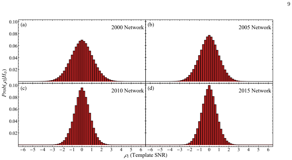
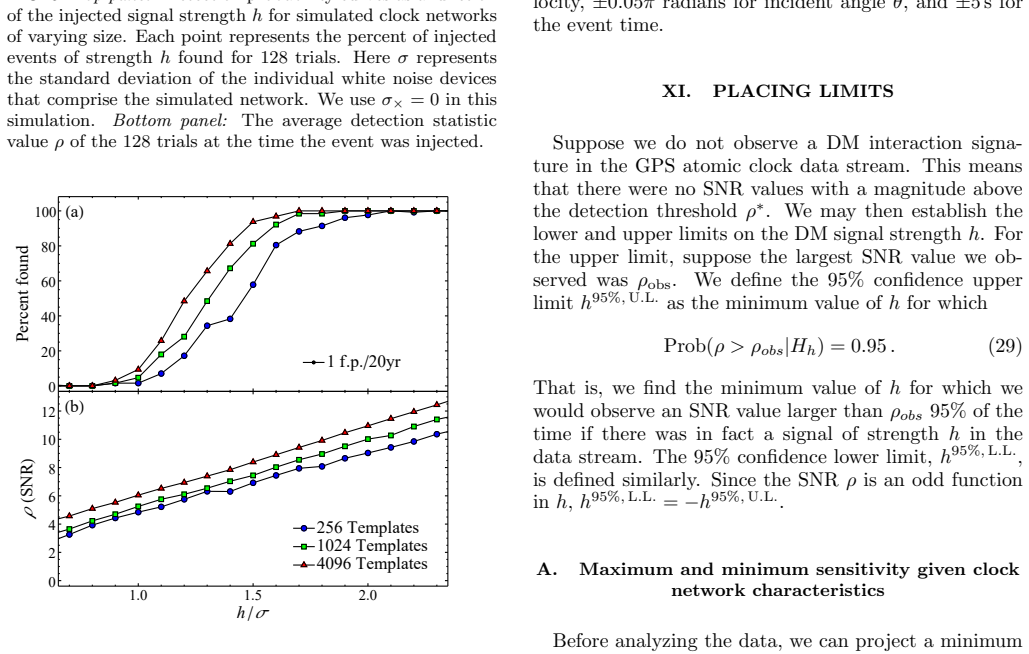
On its own terms, the paper establishes a frequentist detection recipe for dark-matter transients in networks of precision clocks. For an idealized network of $N_D$ identical white-noise sensors sharing a common reference clock, the matched-filter SNR $\rho = d^{T}E^{-1}s/\sqrt{s^{T}E^{-1}s}$ is Gaussian with unit variance and mean $\mu_{\rho} = (h\sqrt{N_D}/\sigma)\sqrt{(1+\eta^2+\xi)/(1+\xi)}$, where $h$ is the strength of the dark-matter-induced clock jump, $\eta$ the ratio of the signal on the reference clock to that on the satellites, and $\xi = N_D\sigma_{\times}^2/\sigma^2$ the relative noise power of the shared reference (Eqs. 24-25). The unit variance is proven for arbitrary covariance structure, so the statistic is self-calibrating even for colored noise and unknown cross-node correlations. In Monte Carlo simulations against realistic GPS constellations from 2000, 2005, 2010, and 2015, the pipeline detects injected thin-domain-wall signals with 95% probability at $h\approx 0.045$ ns on the 2010 network, recovers the event's velocity, direction, and arrival time, and projects discovery reach for dark-matter couplings comparable to laboratory optical-clock limits.
Load-bearing premise
The load-bearing premise is that the clock noise is completely and stably described by the covariance matrix built from prior GPS data, with the shared reference clock as the only source of correlation between satellites; if the differenced noise drifts over the archive or hides additional environmental correlations, the unit-variance calibration and every tabulated threshold in Table II cease to hold.
Editorial extensions
If this is right
- The two decades of archival GPS timing records become searchable as a calibrated frequentist dark-matter experiment, with explicit SNR thresholds for one false positive per day, ten per year, or one per 20 years for each network generation (Table II).
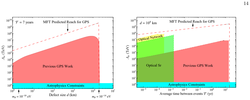
- The matched filter reaches 95% detection probability for thin-wall clock jumps around 0.045 ns on the 2010 constellation, a reach that extends the earlier GPS domain-wall analysis, which was limited to signals well above the instrument noise, by orders of magnitude.
- Sensitivity scales as $\sqrt{N_D}$ with the number of clocks and as $\sqrt{N_E}$ with the number of independent encounters stacked in the search window, so the growing multi-constellation GNSS clock fleet directly strengthens the search.
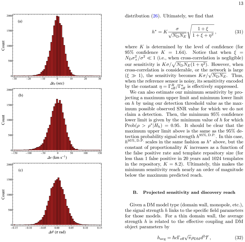
- A detected event carries enough information to reconstruct its velocity ($\pm 27$ km/s), direction ($\pm 0.05\pi$ rad), and time ($\pm 5$ s), enabling a standard-halo-model consistency veto; a null result instead converts into exclusion limits on dark-matter couplings to electrons, quarks, and the fine-structure constant at energy scales comparable to optical-clock constraints.
Reading between the lines
- A natural extension the paper leaves implicit: the same SNR statistic and unit-variance calibration apply to any sensor network whose channels share a common reference or common environmental noise, so ground-based clock networks and magnetometer arrays could reuse the pipeline as-is instead of deriving a new covariance model.
- The sharpest untested premise is stationarity, so the single most informative follow-up is empirical: compute $\sigma_\rho$ on rolling segments of the real archive; if it wanders, per-segment recalibration of the thresholds would be needed before any claim of a 20-year false-alarm rate.
- Because the SNR is an odd function of the signal strength, the same pipeline natively covers both signs of the dark-matter coupling (clocks speeding up or slowing down); a positive detection would let the mixed Rb/Cs/H-maser network disentangle which fundamental constant shifts, through the distinct coefficient combinations the paper tabulates.
- The analytic mean neglects the fractional degeneracy $\lambda$ of two satellites being hit within the same 30-second epoch; as future constellations grow denser, $\lambda$ will rise, and the Gaussian calibration of the statistic would need to be revisited at that point.
Signed reviews
Editorial analysis
A structured set of objections, weighed in public.
Referee Report
Summary. This paper develops a frequentist matched-filter search for transient dark-matter signals, specifically thin domain walls, in networks of precision sensors with a common reference clock, using GPS atomic clock data as the target application. The authors define a template-specific SNR (Eq. 20), construct thin-wall signal templates with an importance-sampled template bank, and derive analytic Gaussian statistics for an idealized network of identical white-noise sensors with a common white-noise reference (mean in Eq. 24, unit variance in Eq. 25). They prove the unit-variance property in Appendix B.1, compute false-positive thresholds for four GPS network configurations (Table II), and use Monte Carlo simulations to estimate 95% detection probabilities (for example, h95%=0.045 ns for the 2010 network) and parameter-extraction resolutions. The paper closes with projected exclusion limits on DM couplings. The calibration is carried out entirely on simulated GPS noise; the pipeline is not applied to archival GPS data.
Significance. The analytic derivation is clean, and the unit-variance proof in Appendix B.1 is a genuinely useful contribution that extends matched-filter treatments to networks with cross-node correlated noise. The Monte Carlo checks, including the 94.6% versus 95% detection-probability agreement in Sec. IX B, are consistent with the Gaussian predictions. If the calibration survives contact with real GPS noise, the method offers a calibrated frequentist complement to the Bayesian search of Ref. [14] and gives concrete projected sensitivity estimates. The main open question is not the internal mathematics but whether the simulated-noise assumptions support the stated false-positive thresholds and detection probabilities for archival use.
major comments (3)
- [Sec. VIII A and Appendix A2, Table III] As written, Section VIII states that the simulations use the perturbative inverse of the covariance matrix, and Appendix A2 states that the von Neumann expansion converges only when the relevant eigenvalues are smaller than unity. For the 2010 operating point quoted in Sec. XI B (sigma ~ 0.02 ns, sigma_x ~ 0.006 ns, ND = 33), the expansion parameter is xi = ND (sigma_x/sigma)^2 ~ 3, so the stated convergence condition is violated. Table III shows the approximation already produces sigma_rho = 8.96 at sigma_x/sigma = 0.5 (xi ~ 7.5 for ND = 30), and the paper does not test the 2010 value sigma_x/sigma ~ 0.3. If the simulations indeed used the perturbative inverse, the Table II thresholds and the Fig. 4 h95% = 0.045 ns value for 2010 are not established; the authors should recompute them with the exact inverse or demonstrate that the perturbative inverse is valid for their heterogeneous 2010 network. If the simulations instead used exact Cholesky inversion, the text should say so explicitly.
- [Sec. VIII and Sec. IX] The null calibration and detection thresholds are obtained entirely from simulated noise generated from prior power spectral densities plus a white common reference clock (Sec. V A), with no validation on archival GPS data. The paper presents thresholds for one false positive in 20 years (Table II) and reports h95% for the 2010 network (Sec. IX B), but it never applies the pipeline to a real, signal-free GPS segment to check that template-specific SNRs are Gaussian with the simulated sigma_rho values or that the max-statistic false-positive rate matches Table II. Real GPS noise is nonstationary (clock swaps, satellite maneuvers, environmental correlations), so the calibration of the proposed archival search is unsupported. The authors should either add null-data validation or explicitly rescope the claims to simulated data only.
- [Eq. (27), Sec. VIII] The false-positive probability per epoch treats the M template-specific SNRs as independent. Because templates are drawn from continuous priors over velocity, direction, and arrival time, neighboring templates will produce correlated SNRs, so the distribution of the maximum statistic defined in Eq. (21) need not follow Eq. (27). The paper verifies only the marginal distribution of individual template SNRs in Fig. 2, not the false-positive rate of the actual detection statistic. Without a Monte Carlo characterization of the max statistic under H0, the thresholds in Table II are not fully calibrated even within the simulated-noise model.
minor comments (4)
- [Sec. V] The word 'whitten' in 'we "whitten" the data' appears to be a typo for 'whiten'.
- [Sec. II] The sentence 'geophysicists were been able to identify' contains a grammatical error and should read 'were able to identify'.
- [Eq. (24) and Eq. (B8)] The main text should note explicitly that Eq. (24) drops the fractional-degeneracy factor lambda that appears in the exact expression (B8), and should comment on the size of this approximation for GPS.
- [Reference [45]] Reference [45] has an incomplete arXiv identifier ('arXiv preprint arXiv: . . . 10, 582 (2013)') and should be completed.
Circularity Check
No significant circularity: the analytic SNR results and detection thresholds are derived from the noise covariance and validated by simulation; cited prior GPS noise work is grounded in archival-data comparison.
full rationale
The paper's central derivation (Secs. VII and Appendix B) computes the matched-filter SNR distribution from the definition of the statistic (Eq. 20), the assumed signal template (Eq. 22), and the covariance matrix (Eqs. A4/A10). The unit-variance property (Eq. 25) is a mathematical identity following from the normalization of the SNR and the definition of the covariance matrix (Appendix B 1), not a fitted prediction. The detection thresholds (Table II) are Monte Carlo quantiles of the null distribution obtained from simulated data generated using independently documented GPS power spectral densities and a common reference clock model (Sec. V A), with no parameter adjusted to a target dark-matter signal. The projected sensitivity (Eq. 31, Fig. 9) uses the analytic SNR mean with network parameters (ND, sigma, sigma_x) and the thin-domain-wall signal model from prior work; this is a forward calculation, not an inversion of data into a result. Self-citations to Refs. [13,14] supply the noise model and the DM signal model, but Ref. [14] is described as including direct comparison to GPS archival data, so it is externally grounded rather than a circular premise. The auxiliary simulation in Sec. IX B that injects h_95% and recovers 94.6% detection is an internal consistency check, not a circular derivation. The absence of a real-data null validation is a correctness/robustness concern, not a circularity concern.
Assumptions & free parameters
free parameters (2)
- Template repository size M =
1024 (256 and 4096 also tested)
- Fractional degeneracy lambda =
approximately 0.2
assumptions (4)
- domain assumption The differenced GPS clock pseudo-frequency noise is stationary, Gaussian, and fully characterized by known power spectral densities, with the reference clock as the only common cross-node noise source.
- domain assumption The covariance matrix can be estimated from the data itself because dark matter events are rare enough not to bias the noise estimate.
- domain assumption The thin-domain-wall transient has the delta-function differenced-data shape of Eq. (22), with the reference clock receiving a scaled opposite spike, and only one event occurs per search window.
- domain assumption The standard halo model provides the quasi-Maxwellian velocity priors and event-rate assumptions used for template generation and projected sensitivity.
Cite this review
Pith. "Pith review of Applying the matched-filter technique to the search for dark matter transients with networks of quantum sensors." pith.science (2026). https://pith.science/paper/CB5VMKMW
@misc{pith2026190803320,
  author       = {Pith},
  title        = {Pith review of: Applying the matched-filter technique to the search for dark matter transients with networks of quantum sensors},
  year         = {2026},
  howpublished = {\url{https://pith.science/paper/CB5VMKMW}},
  note         = {Machine review of arXiv:1908.03320}
}
read the original abstract
There are several networks of precision quantum sensors in existence, including networks of atomic clocks, magnetometers, and gravitational wave detectors. These networks can be re-purposed for searches of exotic physics, such as direct dark matter searches. Here we explore a detection strategy for macroscopic dark matter objects with such networks using the matched-filter technique. Such "clumpy" dark matter objects would register as transients sweeping through the network at galactic velocities. As a specific example, we consider a network of atomic clocks aboard the Global Positioning System (GPS) satellites. We apply the matched-filter technique to simulated GPS atomic clock data and study its utility and performance. The analysis and the developed methodology have a wide applicability to other networks of quantum sensors.
Figures

Figures from the paper (5 more)


Reference graph
Works this paper leans on
-
[14]
R. M. Godun, P. B. R. Nisbet-Jones, J. M. Jones, S. A. King, L. A. M. Johnson, H. S. Margolis, K. Szymaniec, S. N. Lea, K. Bongs, and P. Gill, Phys. Rev. Lett. 113, 210801 (2014)
2014
-
[1]
Here subscripts j and l range over epochs and the superscripts a and b span network sensors
Properties of the network covariance matrix The covariance matrixE is given by the ensemble av- erage Eab jl =⟨na jnb l⟩≡ E(aj)(bl), (A1) wherena j is the noise in the datastream of thea-th device at the temporal grid point (epoch) j, and ⟨na j⟩ = 0 is assumed. Here subscripts j and l range over epochs and the superscripts a and b span network sensors. Wh...
work page 2015
-
[2]
Perturbative inversion This approximation to inverting the network covari- ance matrix was used in our earlier GPS.DM work [14] and we will detail it below. It relies on the von Neumann series expansion, (G +λF )−1 =G−1 ∞∑ n=0 (−1)nλn( FG−1)n ≈G−1−λG−1FG−1, (A11) where G and F are matrices and λ is the expansion (book-keeping) parameter. This identity can...
work page 2015
-
[3]
Performance comparison between exact and perturbative inversion In order to utilize the perturbative inversion outlines in the above section, we require that the reference de- vice noise be sufficiently smaller than that of the node devices. To verify the inadequacy of the perturbative 17 inversion for networks with a noisy reference sensor, we simulated si...
-
[4]
SNR variance The goal of this section is to prove that Var{dTE−1s} =sTE−1s, implying that the SNR variance (B9) is σ2 ρ = 1. The proof holds regardless of the nature of the covariance ma- trix - for example it applies to colored noise network with arbitrary cross-node correlations. Explicitly, Var{dTE−1s} = ⟨( nTE−1s )( nTE−1s )⟩ , wheren is the intrinsic...
- [5]
-
[6]
C. L. Degen, F. Reinhard, and P. Cappellaro, Rev. Mod. Phys. 89, 035002 (2017), arXiv:1611.02427
arXiv 2017
-
[7]
M. S. Safronova, D. Budker, D. DeMille, D. F. J. Kimball, A. Derevianko, and C. W. Clark, Rev. Mod. Phys. 90, 025008 (2018)
2018
Show all 50 references
-
[8]
Vilenkin, Phys
A. Vilenkin, Phys. Rep. 121, 263 (1985)
1985
-
[9]
Coleman, Nucl
S. Coleman, Nucl. Phys. B 262, 263 (1985)
1985
-
[10]
Kusenko, Phys
A. Kusenko, Phys. Rev. Lett. 87, 141301 (2001)
2001
-
[11]
K. Lee, J. A. Stein-Schabes, R. Watkins, and L. M. Widrow, Phys. Rev. D 39, 1665 (1989)
1989
-
[12]
J. Liu, X. Chen, and X. Ji, Nature Physics 13, 212 (2017)
2017
-
[13]
Huntemann, B
N. Huntemann, B. Lipphardt, C. Tamm, V. Gerginov, S. Weyers, and E. Peik, Phys. Rev. Lett. 113, 210802 (2014)
2014
-
[15]
Pospelov, S
M. Pospelov, S. Pustelny, M. P. Ledbetter, D. F. J. Kim- ball, W. Gawlik, and D. Budker, Phys. Rev. Lett. 110, 021803 (2013)
2013
-
[16]
Derevianko and M
A. Derevianko and M. Pospelov, Nature Physics 10, 933 (2014), arXiv:1311.1244
2014 arXiv
-
[17]
B. M. Roberts, G. Blewitt, C. Dailey, M. Murphy, M. Pospelov, A. Rollings, J. Sherman, W. Williams, and A. Derevianko, Nature Communications 8, 1195 (2017), arXiv:1704.06844
2017 arXiv
-
[18]
B. M. Roberts, G. Blewitt, C. Dailey, and A. Derevianko, Phys. Rev. D 97, 83009 (2018), arXiv:1803.10264
2018 arXiv
-
[19]
Wcis lo, P
P. Wcis lo, P. Ablewski, et al. , Science Advances 4, eaau4869 (2018)
2018
-
[20]
J. D. Romano and N. J. Cornish, Living Reviews in Rel- ativity 20, 1 (2017), arXiv:1608.06889
2017 arXiv
-
[21]
F. Dong, E. Pierpaoli, J. Gunn, and R. Wechsler, Astro- phys. J. 676, 868 (2008)
2008
- [22]
-
[23]
Auger, D
M. Auger, D. Auty, et al. , Phys. Rev. Lett. 109 (2012), 10.1103/PhysRevLett.109.032505
2012 doi
-
[24]
Abbott et al
B. Abbott et al. , Phys. Rev. Lett. 116 (2016), 10.1103/PhysRevLett.116.061102
2016 doi
- [25]
-
[26]
Bovy and S
J. Bovy and S. Tremaine, Astrophys. J. 756, 89 (2012)
2012
-
[27]
Wcis lo, P
P. Wcis lo, P. Morzy´ nski, M. Bober, A. Cygan, D. Lisak, R. Ciury lo, and M. Zawada, Nature Astronomy 1, 0009 (2016)
2016
-
[28]
Sikivie, Phys
P. Sikivie, Phys. Rev. Lett. 48, 1156 (1982)
1982
-
[29]
Press, B
W. Press, B. Ryden, and D. Spergel, Astrophys. J. 347, 590 (1989)
1989
-
[30]
Vilenkin and E
A. Vilenkin and E. P. S. Shellard, Cosmic Strings and Other Topological Defects (Cambridge University Press, 2000)
2000
-
[31]
Durrer, M
R. Durrer, M. Kunz, and A. Melchiorri, Phys. Rep. 364, 1 (2002)
2002
-
[32]
Friedland, H
A. Friedland, H. Murayama, and M. Perelstein, Phys. Rev. D 67, 043519 (2003)
2003
-
[33]
P. P. Avelino, C. J. A. P. Martins, J. Menezes, R. Menezes, and J. C. R. E. Oliveira, Phys. Rev. D 78, 103508 (2008)
2008
-
[34]
Marsh and A
D. Marsh and A. Pop, Mon. Not. Roy. Astron. Soc. 451, 2479 (2015)
2015
-
[35]
Schive, T
H.-Y. Schive, T. Chiueh, and T. Broadhurst, Nature Physics 10, 496 (2014)
2014
-
[36]
Hogan and M
C. Hogan and M. Rees, Phys. Lett. B 205, 228 (1988)
1988
-
[37]
E. W. Kolb and I. I. Tkachev, Phys. Rev. Lett. 71, 3051 (1993)
1993
-
[38]
D. M. Grabowska, T. Melia, and S. Rajendran, Phys. Rev. D 98, 115020 (2018), arXiv:1807.03788
2018 arXiv
-
[39]
V. A. Dzuba, V. V. Flambaum, and M. V. Marchenko, Phys. Rev. A 68, 022506 (2003)
2003
-
[40]
V. V. Flambaum and A. F. Tedesco, Phys. Rev. C 73, 055501 (2006)
2006
-
[41]
Savalle, B
E. Savalle, B. M. Roberts, F. Frank, P.-E. Pottie, B. T. McAllister, C. B. Dailey, A. Derevianko, and P. Wolf, (2019), arXiv:1902.07192
2019 arXiv
-
[42]
Wcis lo, P
P. Wcis lo, P. Ablewski, K. Beloy, S. Bilicki, M. Bober, R. Brown, R. Fasano, R. Ciury lo, H. Hachisu, T. Ido, J. Lodewyck, A. Ludlow, W. McGrew, P. Morzy´ nski, D. Nicolodi, M. Schioppo, M. Sekido, R. Le Targat, P. Wolf, X. Zhang, B. Zjawin, and M. Zawada, Science Advances 4,...
2018
-
[43]
B. M. Roberts, G. Blewitt, C. Dailey, M. Murphy, M. Pospelov, A. Rollings, J. Sherman, W. Williams, and A. Derevianko, Nature Comm. 8, 1195 (2017)
2017
-
[44]
Blewitt, Treatise on Geophysics (Elsevier, Oxford,
G. Blewitt, Treatise on Geophysics (Elsevier, Oxford,
-
[45]
Data freely available online: Jet Propulsion Laboratory ftp://sideshow.jpl.nasa.gov/pub/jpligsac/
-
[46]
Rollings, Undergraduate Thesis (2016)
A. Rollings, Undergraduate Thesis (2016)
2016
-
[47]
GNSS constellation status online: European GNSS Service Centre https://www.gsc-europa.eu/ system-status/Constellation-Information
-
[48]
K. A. Olive and M. Pospelov, Phys. Rev. D 77, 043524 (2008)
2008
-
[49]
K´ om´ ar, E
P. K´ om´ ar, E. Kessler, and M. Bishof, arXiv preprint arXiv: . . . 10, 582 (2013)
2013
-
[50]
K´ om´ ar, T
P. K´ om´ ar, T. Topcu, E. M. Kessler, A. Derevianko, V. Vuleti´ c, J. Ye, and M. D. Lukin, Phys. Rev. Lett. 117, 60506 (2016)
2016
Reviewed August 14, 2026 · model on record in the stance chip above.
Discussion (0). Continue with ORCID to comment.