REVIEW 2 major objections 5 minor 36 references
Quantum Traversal Time Across a Potential Well
T0 review · 2 major / 5 minor · reviewed 2026-08-14 · deepseek-v4-flash
Pith's one-line read The paper derives a closed-form expression for the quantum traversal time across a potential well and shows that for deep wells the time can be negative, so the packet is advanced or delayed.
desk verdict A genuine extension of the TOA traversal-time program with a novel closed-form result, but the key quantum term rests on an unproved residue cancellation that needs to be fixed before the deep-well predictions can be trusted. read the letter →
The pith
A machine-rendered reading of the paper's core claim, the machinery that carries it, and where it could break.
The reading
What carries the argument
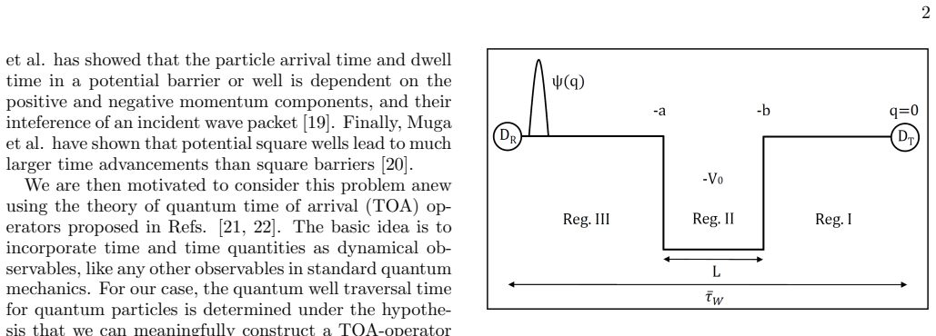
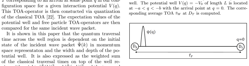
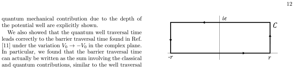
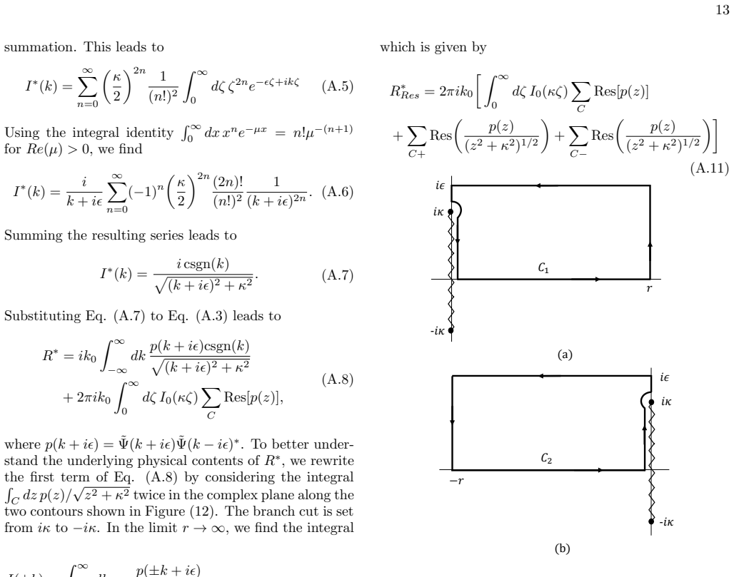
The object that carries the argument is the time-of-arrival operator $\hat T$, obtained by quantizing the classical arrival time; for the free particle its kernel is $T_F(q,q')=(q+q')/4$, while for the well the kernel is built in three spatial regions and contains modified Bessel functions, with $\tilde T_3(\eta,\zeta)=\eta/2-(L/2)[I_0(\kappa|\zeta|)-1]$ for packets whose support starts left of the well. The traversal time is the difference $\langle \hat T_F\rangle-\langle \hat T_W\rangle$, which reduces to $\tau_W=(L/v_0)R$, where $R$ is an effective index of refraction obtained as the imaginary part of the double integral $R^*=k_0\int_0^\infty d\zeta I_0(\kappa\zeta)\int dk|\Psi(k)|^2 e^{ik\zeta}$. The decisive step is the evaluation of this integral in the complex plane: the paper uses the identity $\int_0^\infty d\zeta I_0(\kappa\zeta)e^{i(k+i\epsilon)\zeta}=i\,\mathrm{csgn}(k)/\sqrt{(k+i\epsilon)^2+\kappa^2}$ for $\epsilon>\kappa$, then deforms contours to obtain the three-term decomposition and, for arbitrary states, the asserted cancellation of residue contributions.
What would settle it
Choose a Gaussian incident packet with parameter values in the region where Eq. (51) predicts a negative index $R$, and evaluate the original double integral $R^*=k_0\int_0^\infty d\zeta I_0(\kappa\zeta)\int_{-\infty}^\infty dk|\Psi(k)|^2e^{ik\zeta}$ numerically with a convergence factor $e^{-\epsilon\zeta}$ for $\epsilon>\kappa$, then analytically continue to $\epsilon\to0^+$. If the regulated value does not match Eq. (26) — in particular, if it is nonnegative where the paper predicts a sign change — the complex-plane reduction is not correct and the negative-traversal-time prediction fails.
Extended reading notes
Core claim
The central claim is that the expected quantum traversal time across a well of depth $V_0$ and width $L$ has the exact three-term form $$ \tau_W=\int_0^\infty dk\,\tau_{\mathrm{top}}(k)|\Psi(k)|^2-\int_0^\infty dk\,\tau_{\mathrm{top}}(k)|\Psi(-k)|^2-\int_0^\kappa dk\,\tau_{\mathrm{in}}(k)\operatorname{Im}[2\Psi(ik)\Psi^*(-ik)], $$ with $\kappa=\sqrt{2\mu V_0}/\hbar$, $\tau_{\mathrm{top}}(k)=L/v_{\mathrm{top}}(k)$, $\tau_{\mathrm{in}}(k)=L/v_{\mathrm{in}}(k)$, $v_{\mathrm{top}}(k)=\hbar\sqrt{k^2+\kappa^2}/\mu$, and $v_{\mathrm{in}}(k)=\hbar\sqrt{\kappa^2-k^2}/\mu$. The first two terms are classical weighted averages with momentum probabilities $|\Psi(\pm k)|^2$; the third term is purely quantum, supported for $0\le k\le\kappa$, and its weight is an imaginary cross-term rather than a probability. The paper argues that for deep wells this third term dominates and oscillates, so $\tau_W$ can be negative; it further shows that the same formula analytically continues to the barrier case under $V_0\to -V_0$, where the quantum term cancels the sub-barrier contribution and reproduces the known instantaneous-tunneling result.
Load-bearing premise
The result depends on the unproved assertion that the complex-plane evaluation of the double integral is valid, including the exact cancellation of boundary and residue terms that leaves only the three terms of Eq. (27); if that cancellation fails, the purely quantum contribution to the traversal time, and with it the deep-well negative traversal times, does not follow.
Editorial extensions
If this is right
- For shallow wells ($\kappa/k_0\to0$) and spatially broad packets, $\tau_W$ approaches the classical well traversal time with small quantum corrections governed by the packet width; the correspondence-principle limit is recovered as $\hbar\to0$.
- For shallow wells and narrow packets, $\tau_W$ approaches the free-particle quantum traversal time plus corrections controlled by $\kappa$, so a weak well acts as a perturbation to free propagation.
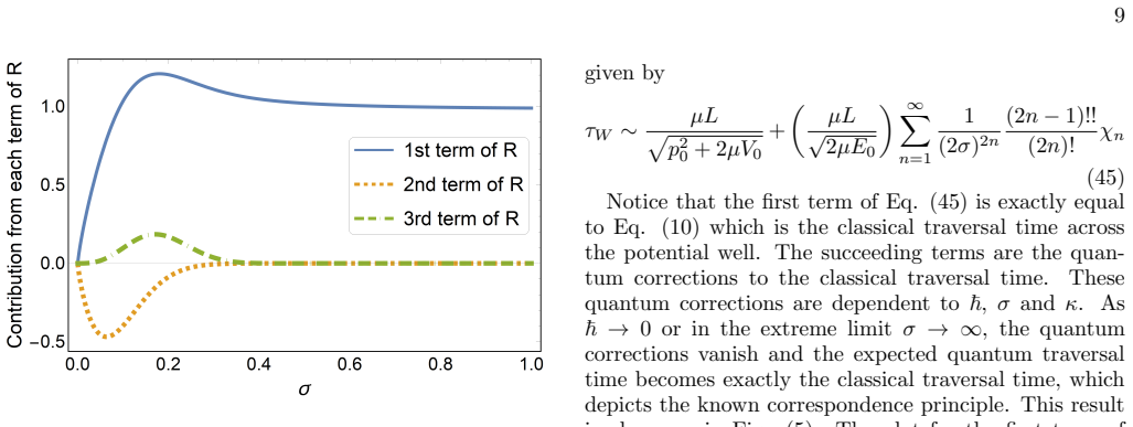
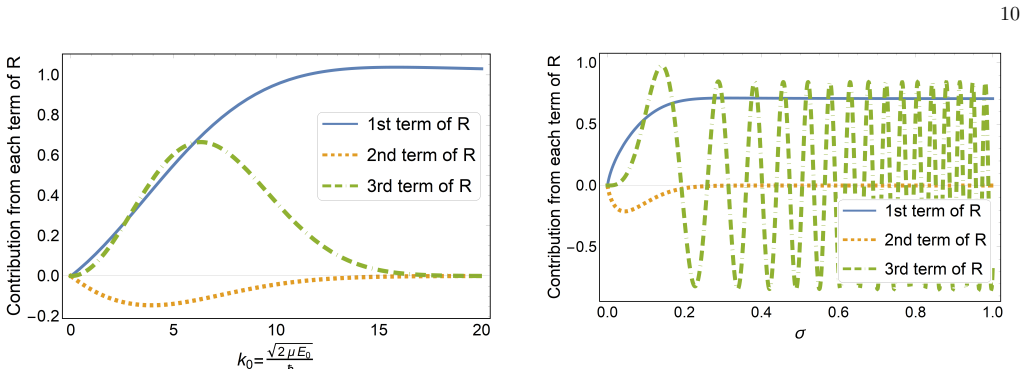
- For deep wells ($\kappa/k_0\to\infty$), the third term dominates and $\tau_W$ oscillates from positive to negative; the sign is determined by $\sigma k_0$ and $\sigma\kappa$, so shaping the packet or well depth can switch between delay and advance.
- Analytically continuing $V_0\to -V_0$ turns the well traversal time into the barrier traversal time; sub-barrier momentum components then contribute zero traversal time, recovering instantaneous tunneling as a limiting case.
Reading between the lines
- Inference: a direct numerical evaluation of the original double integral with an $\epsilon>\kappa$ regulator and analytic continuation to $\epsilon\to0$ would independently test the complex-plane reduction for the Gaussian packets of Sec. V, without relying on the paper's contour argument.
- Inference: the same complex-plane decomposition should apply to smooth or asymmetric wells; if the sign-indefinite quantum term survives there, the effect is a general feature of quantum traversal time rather than an artifact of rectangular edges.
- Inference: because the paper ties the negative traversal time to negative group velocity and reflection, a classical-wave experiment at parameters where Eq. (27) predicts a sign change could separate genuine advancement from reflection loss and sharpen the operational meaning of negative traversal time.
Signed reviews
Editorial analysis
A structured set of objections, weighed in public.
Referee Report
Summary. The manuscript constructs a quantum time-of-arrival (TOA) operator for a one-dimensional rectangular potential well via Weyl quantization and defines the expected traversal time as the difference between the expectation values of the free and well TOA operators. The central result is Eq. (27), which expresses the well traversal time as the sum of two classical-like weighted contributions from positive and negative momentum components and a third purely quantum contribution involving the incident wave function at imaginary momenta. For a Gaussian wave packet, the authors find that shallow wells reproduce the classical and free-particle traversal times in appropriate limits, while deep wells yield an oscillatory traversal time that can be negative, implying advanced or delayed arrival. The derivation of Eq. (27) relies on a contour-integral evaluation in Appendix A.
Significance. If the technical gaps are resolved, this would be a novel addition to the quantum time-of-arrival literature. The expression (27) is derived from first principles rather than fitted, and it passes several internal consistency checks: it reduces to the known barrier traversal time under V0→−V0 (Sec. IV), to the classical well traversal time in the high-energy limit (Eqs. 19-20), and to the free-particle traversal time for narrow wave packets (Sec. V.A). The paper explicitly separates classical and quantum contributions, which is a useful feature. However, the significance is conditional on the missing proof of the residue cancellation and analytic continuation in Appendix A.
major comments (2)
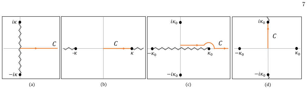
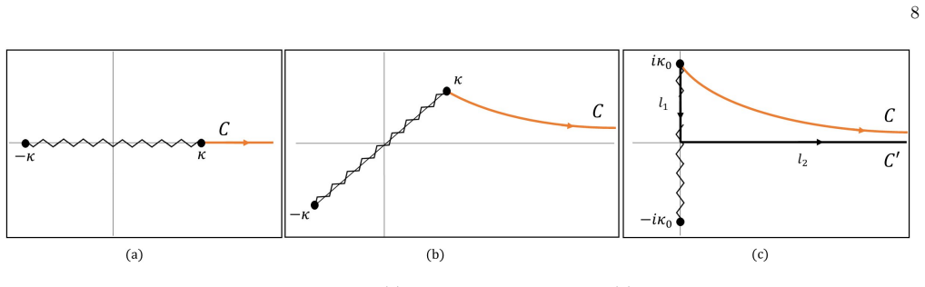
- [Appendix A, Eq. (A.11)] The assertion that 'the first term of Eq. (A.11) cancels the second and third terms so that R*_Res = 0' is made without proof. This cancellation is the step that removes the pole contributions and leaves the pure integral form of Eq. (A.10), which in turn yields the third term of Eq. (27). The analytic continuation from ϵ>κ (where Eq. (A.3) converges) to the physical ϵ<κ regime is also not justified. In addition, the step from Eq. (A.8) to Eq. (A.10) via Eq. (A.9) involves a contour deformation whose signs and branch-cut contributions are not derived. Please provide a rigorous derivation or a numerical verification of the cancellation and the continuation.
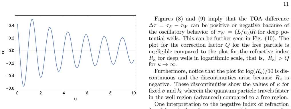
- [Sec. V.B, Eqs. (39)-(40)] The transformation from Eq. (39) to Eq. (40) is stated without any derivation ('Equation (39) is rewritten by lifting the integral in the complex plane', no details). The deep-well analysis, including the exponentially large factor e^{2σ²(κ²−k0²)} and the oscillatory factor in z, depends entirely on this rewriting. Without a proof of the contour deformation and the resulting expressions for z and γ, the prediction of oscillatory negative traversal times for deep wells is not established.
minor comments (5)
- [Eq. (9), t2] For a particle initially inside the well (region II), the classical time to reach the origin should involve momentum sqrt(p0²+2µV0) for the segment inside the well and p0 for the free segment; Eq. (9) appears to have these reversed, and the condition 2µV0/p0²<1 is appropriate only for a barrier. Please correct or clarify.
- [Sec. II, after Eq. (6)] The claim that the time kernels are equal for Weyl, Born-Jordan, and simple symmetric quantizations is stated without proof; provide a reference or a brief derivation.
- [Figure 2 caption] The caption contains the typo 'abscence'; it should be 'absence'.
- [Sec. V.B] The word 'microelectrenonics' should be 'microelectronics'.
- [Eq. (44)] The notation d(2n)/dk(2n) is nonstandard; use d^{2n}/dk^{2n} for the 2n-th derivative.
Circularity Check
No circularity: Eq. (27) is derived from the TOA-operator quantization and checked against independent classical, free-particle, and barrier limits; the Appendix A cancellation is an unproved step, not an equivalence-by-construction.
full rationale
The derivation is self-contained once the TOA-operator framework is granted. Eq. (27) is obtained from Eq. (25) by the complex-plane reduction in Appendix A: the first two terms are the real-axis contributions and the third is the imaginary-axis contribution. Nothing in this reduction is fitted to data, nor is the target traversal time defined in terms of the result. The checks against the classical limit (Eqs. (9)-(10) and (43)-(45)), the free-particle traversal time (Eq. (50)), and the barrier traversal time (Eqs. (28)-(30)) are consistency checks against independent limiting results, not inputs. The paper's many self-citations (Refs. [11,21,22,25,26,27,29,30]) supply the TOA-operator quantization scheme and earlier limiting results; these are framework assumptions that do not include the well traversal time formula, so they do not make the derivation circular. The genuinely load-bearing mathematical assertion that the residue contribution vanishes, stated in Appendix A as 'It turns out that the first term of Eq. (A.11) cancels the second and third terms so that R*_Res = 0', is unproved, and the analytic continuation from ϵ>κ to the physical ϵ<κ regime is asserted rather than demonstrated. This is a missing proof and a correctness risk for the deep-well oscillation claim, but it is not a case of the prediction reducing to its input by construction or of a fitted parameter being renamed as a prediction. Therefore, no circular step is exhibited.
Assumptions & free parameters
assumptions (5)
- domain assumption The TOA operator defined by Eq. (3) via Weyl quantization is the correct quantum observable for arrival time at a point, and its expectation value computes the average arrival time in the measurement scheme.
- domain assumption The expectation value Im(τ*) corresponds to the operational arrival time even though the measurement post-selects on detected particles.
- domain assumption The incident wave packet is infinitely differentiable with support strictly to the left of the well.
- ad hoc to paper The contour deformations and analytic continuation in Appendix A are valid, and the residue contributions cancel (R*_Res = 0).
- domain assumption For constant piecewise potentials, the time kernels are equal for Weyl, Born-Jordan, and simple symmetric quantizations.
Cite this review
Pith. "Pith review of Quantum Traversal Time Across a Potential Well." pith.science (2026). https://pith.science/paper/CF5MGO5M
@misc{pith2026190803400,
  author       = {Pith},
  title        = {Pith review of: Quantum Traversal Time Across a Potential Well},
  year         = {2026},
  howpublished = {\url{https://pith.science/paper/CF5MGO5M}},
  note         = {Machine review of arXiv:1908.03400}
}
read the original abstract
We consider the quantum traversal time of an incident wave packet across a potential well using the theory of quantum time of arrival (TOA)-operators. This is done by constructing the corresponding TOA-operator across a potential well via quantization. The expectation value of the potential well TOA-operator is compared to the free particle case for the same incident wave packet. The comparison yields a closed-form expression of the quantum well traversal time which explicitly shows the classical contributions of the positive and negative momentum components of the incident wave packet and a purely quantum mechanical contribution significantly dependent on the well depth. An incident Gaussian wave packet is then used as an example. It is shown that for shallow potential wells, the quantum well traversal time approaches the classical traversal time across the well region when the incident wave packet is spatially broad and approaches the expected quantum free particle traversal time when the wave packet is localized. For deep potential wells, the quantum traversal time oscillates from positive to negative implying that the wave packet can be advanced or delayed.
Figures
Figures from the paper (8 more)


Reference graph
Works this paper leans on
-
[1]
J. G. Muga, R. S. Mayato, I. L. Egusquiza eds., Time in Quantum Mechanics, Vol 1 (Springer, Berlin, 2008)
work page 2008
-
[2]
(42) One immediately notices from Eq
Im(z) +e−2σ2k2 0γ ] (40) where z =e4iσ2k0κ ∫ ∞ 0 idk e−2σ2(k2+2k0k)e4iσ2κk √ k2− 2iκk , (41) γ = ∫ ∞ 0 dke−2σ2(k2−2k0k) √ k2 +κ2 . (42) One immediately notices from Eq. (39) that the third term of R approaches 0 as κ→ 0. However, this be- comes dominant when κ→∞ , σ→∞ when κ > k0, or both as can be seen from Eq. (40) because of the exponentially large fac...
-
[3]
Since σ is very small, our momentum distribution is broad and we can no longer neglect the contributions from the second and third terms in Eq. (26) as we did previously. This can be verified if we plot R as shown in Fig. (6). The third term of Eq. (26) significantly contributes to the effective index of refraction of the well when κ/k0≤ 1 but becomes subdom...
-
[4]
Im(z), (51) where z is given by Eq. (41). For convenience, we change variables to u = σκ and v = σk0 and numerically solve z. One can already no- tice that R oscillates from positive to negative for deep potential wells because of the presence of the complex exponential e4iσ2k0κ in Eq. (41). This can be further seen from the 2d and 3d plots of the imagina...
-
[5]
under the variation V0→−V0 in the complex plane. In particular, we found that the barrier traversal time can actually be written as the sum involving the classical and quantum contributions, similar to the well traversal time. However, the presumably third term in RB with weight Im [ 2 ˜Ψ(ik) ˜Ψ∗(−ik) ] , which we identified earlier as a purely quantum con...
-
[6]
A. S. Landsman and U. Keller, Phys. Rep. 547 1 (2015)
work page 2015
- [7]
-
[8]
J. G. Muga, A. Ruschhaupt, A. del Campo eds., Time in Quantum Mechanics, Vol 2 (Springer, Berlin, 2009). 14
work page 2009
Show all 36 references
-
[9]
Landauer, and Th
R. Landauer, and Th. Martin, Rev. Mod. Phys. 66 217 (1994)
1994
-
[10]
H. G. Winful, Phys. Rep. 436 1 (2006)
2006
-
[11]
Now, in the absence of the potential well, substituting the time kernel ˜TF (η,ζ ) = η/2 into Eq
and Pollak [13] for the potential barrier case. Now, in the absence of the potential well, substituting the time kernel ˜TF (η,ζ ) = η/2 into Eq. (12) gives the complex- expected TOA for the free particle case given by τ∗ F =−µ ℏ ∫ ∞ 0 ∫ ∞ −∞ ¯ϕ ( η−ζ 2 ) ϕ ( η +ζ 2 ) ηeik0ζdη...
-
[12]
L. A. MacColl, Phys. Rev. 40 621 (1932)
1932
-
[13]
Pollak, J
E. Pollak, J. Phys. Chem. Lett. 8 352 (2017)
2017
-
[14]
Camus, E
N. Camus, E. Yakaboylu, L. Fechner, M. Klaiber, M. Laux, Y. Mi, K. Z. Hatsagortsyan, T. Pfeifer, C. H. Keitel, and R. Moshammer, Phys. Rev. Lett 119 023201 (2017)
2017
-
[15]
for future works. VII. ACKNOWLEDGMENT D.A.L.P. gratefully acknowledges the financial assis- tance from DOST-SEI through ASTHRDP-NSC gradu- FIG. 11. The contour of integration for Eq. (A.1). ate scholarship program. APPENDIX A. Derivation of the index of refraction R of the pote...
-
[16]
U. S. Sainadh, H. Xu, X. Wang, A. Atia-Tul-Noor, W. C. Wallace, N. Douguet, A. Bray, I. Ivanov, K. Bartschat, A. Kheifets, R. T. Sang and I. V. Litvinyuk, Nature 568 75 (2019)
2019
-
[17]
Zhao and M
J. Zhao and M. Lein, Phys. Rev. Lett. 111 043901 (2013)
2013
-
[18]
E. A. Galapon, Phys. Rev. Lett. 108 170402 (2012)
2012
-
[19]
Petersen and E
J. Petersen and E. Pollak, J. Phys. Chem. A 122 3563 (2018)
2018
-
[20]
Petersen and E
J. Petersen and E. Pollak, J. Phys. Chem. Lett. 8 4017 (2017)
2017
-
[21]
C. F. Li and Q. Wang, J. Phys. Lett. A 275 287 (2000)
2000
-
[22]
M.Vetter, A
R. M.Vetter, A. Haibel and G. Nimtz, Phys. Rev. E 63 046701 (2001)
2001
-
[23]
Chen and C
X. Chen and C. F. Li, Phys. Rev. A 68 052105 (2003)
2003
-
[24]
Chen and C
X. Chen and C. F. Li, Europhys. Lett. 82 30009 (2008)
2008
-
[25]
V. F. Los and N. V. Los, Theor. Math. Phys. 177 1706 (2013)
2013
-
[26]
J. G. Muga, I. L. Egusquiza, J. A. Damborenea and F. Delgado, Phys. Rev. A 66 042115 (2002)
2002
-
[27]
E. A. Galapon, J. Math. Phys. 45 3180 (2004)
2004
-
[28]
E. A. Galapon and J. J. P. Magadan, Ann. Phys. 397 278 (2018)
2018
-
[29]
Y. Ban, X. Chen and C.F. Li, Phys. Lett. A 364 76 (2007)
2007
-
[30]
Y. Wang, X. Chen, Y. Ban and C. F. Li, Phys. E 41 399 (2009)
2009
-
[31]
D. L. B. Sombillo and E. A. Galapon, Phys. Rev. A 90 032115 (2014)
2014
-
[32]
D. L. B. Sombillo and E. A. Galapon, Phys. Rev. A 97 062127 (2018)
2018
-
[33]
E. A. Galapon, Phys. Rev. A 80 030102 (2009)
2009
-
[34]
I. M. Gelfand and G. E. Shilov, Generalized Functions, Vol 1 (Academic, New York, 1964)
1964
-
[35]
C. D. Tica and E. A. Galapon, J. Math. Phys. 60 013502 (2019)
2019
-
[36]
E. A. Galapon, Proc. R. Soc. Lond. A 473 20160567 (2017)
2017
Reviewed August 14, 2026 · model on record in the stance chip above.
Discussion (0). Continue with ORCID to comment.