REVIEW 3 major objections 6 minor 28 references
Extending the Davis-Kahan theorem for comparing eigenvectors of two symmetric matrices II: Computation and Applications
T0 review · 3 major / 6 minor · reviewed 2026-08-14 · deepseek-v4-flash
Pith's one-line read This paper shows that the optimal affine-transform Davis–Kahan bound is the solution of a concave-convex fractional program, so it can be computed globally and automatically, always matching or beating the standard Davis–Kahan bound.
desk verdict Solid computational companion to Paper I—affine extended DK bounds as a solvable concave-convex fractional program with real gains over standard DK; the cvx strict-inequality relaxation is the one real gap, acknowledged and empirically handled but not proven. read the letter →
The pith
A machine-rendered reading of the paper's core claim, the machinery that carries it, and where it could break.
The reading
What carries the argument
The load-bearing object is the ratio $\|c_1\Phi+c_0I-\Psi\|_2/\delta_i$, where $\delta_i$ is one of four possible Davis–Kahan eigenvalue-separation gaps that arise from the two interval choices and the sign of $c_1$. The argument proceeds by showing $\delta_i$ is concave (it is a minimum of affine functions of $c_1,c_0$) while the norm denominator is convex, so maximizing the reciprocal ratio is a concave-convex fractional program. The parameter-free transformation $y_1=c_1/t$, $y_2=c_0/t$, $t=1/\|c_1\Phi+c_0I-\Psi\|_2$ converts each subproblem into a convex program with a norm inequality constraint, making the global optimum automatically computable.
What would settle it
Take two small symmetric matrices with known eigendecompositions, compute the true distance $\inf_{R\in O(r)}\|W-VR\|_F$, and solve the four affine subproblems; any reported bound smaller than that true distance would disprove the claim. A more targeted check is to construct a case where the relaxed convex solve violates the strict $\delta_i>0$ constraints, which would mean the reported optimum is not actually feasible for the extended theorem.
Extended reading notes
Core claim
The paper's central claim is that the optimal affine extension of the Davis–Kahan theorem is a well-posed optimization problem. Writing the transformed matrix as $f(\Phi)=c_1\Phi+c_0I$, the bound on the distance between eigenspaces takes the form $c_{n,r}\|f(\Phi)-\Psi\|_2/\delta_i$, where $\delta_i$ is the post-transformation eigenvalue-separation gap. The paper proves each $\delta_i$ is the minimum of two affine functions and hence concave, the denominator is convex, and the numerator is positive on the feasible set, so maximizing the reciprocal ratio is a concave-convex fractional program. A variable substitution turns it into an equivalent convex program, and an iterative parametric algorithm gives the same optimum; the authors use the first because it is a single convex solve. Consequently the tightest affine Davis–Kahan bound is obtained automatically, is always at least as tight as the standard bound (the identity transform is a feasible point), and can give finite values where the standard interval-separation condition fails.
Load-bearing premise
The computation inherits the extended Davis–Kahan inequality from the companion paper, and if that inequality is wrong, the minimized ratio is not a guaranteed upper bound; the practical solver also relaxes strict constraints to non-strict versions and checks feasibility afterward, without a general proof that this always succeeds.
Editorial extensions
If this is right
- For any pair of symmetric matrices satisfying the extended theorem's assumptions, the best affine bound is obtained by solving one convex program per sign/interval case; no parameter search or user tuning is needed.
- The optimized bound is always at least as tight as the standard Davis–Kahan bound, and in the paper's stochastic-blockmodel and spiked-covariance examples it improves on the standard bound, often by about a factor of two.
- When comparing eigenvectors of the largest or smallest eigenvalues, the affine-optimized bound always matches or beats the trivial bound $c_{n,r}$; Proposition 1 proves the cost function approaches 1 as $c_0\to\pm\infty$.
- The method supplies useful finite bounds in comparisons where the standard Davis–Kahan theorem is inapplicable, such as adjacency-matrix versus Laplacian eigenspaces in the stochastic blockmodel, because the transformation creates a positive separation gap.
- The parameter-free and iterative parametric solution routes agree numerically, with the parameter-free route preferred because it solves a single convex problem.
Reading between the lines
- Editorial inference: the same fractional-programming formulation should extend to polynomial transformations of degree two or more: the transformed spectrum is a sum of powers, so each interval endpoint is selected from finitely many orderings, and each selection still yields a ratio of concave/convex type that could be solved by branch-and-bound. This would test whether higher-degree transforms a
- Editorial inference: because the bound is cheap to compute, it could be used as a finite-sample certificate inside spectral clustering or PCA pipelines: if the optimized bound is close to 1, the observed eigenvector space is not yet informative about the population space, giving a data-dependent rule of thumb for when more samples are needed.
- Editorial inference: the spiked-covariance experiments suggest a practical diagnostic that goes beyond the paper: the optimized bound as a function of sample size $N$ could be inverted to choose the minimal $N$ at which the leading-$r$ sample eigenspace is guaranteed close to the population eigenspace at a user-specified tolerance.
Signed reviews
Editorial analysis
A structured set of objections, weighed in public.
Referee Report
Summary. This manuscript is the computational companion to the authors' Paper I, which extended the Davis–Kahan theorem by allowing a polynomial transform of one of the two symmetric matrices. Here the authors specialize to affine transformations and formulate the problem of choosing the affine parameters c1,c0 so as to minimize the extended Davis–Kahan bound as a fractional program. They prove that the relevant separations δ1,+, δ1,−, δ2,+, δ2,− are concave, show that the denominator is convex, and conclude that each of the four subproblems is a concave-convex fractional program for which every local optimum is global. The authors then discuss the Charnes–Cooper transformation and Dinkelbach's algorithm as solution strategies, implement the former in cvx, and apply the method to three examples: comparisons of graph shift operators from stochastic block models, comparisons of graph shift operators with their corresponding generating matrices, and comparisons of sample versus population covariance matrices in a spiked covariance model. The main claims are that the affine-extended Davis–Kahan bound is computable automatically via convex optimization, that it is always at least as tight as the standard Davis–Kahan bound, and that it yields finite informative values in settings where the standard theorem does not apply.
Significance. If the central claim holds, the paper makes a genuinely useful contribution: it turns the extended Davis–Kahan theorem into an automated tool, and the three applications—especially the graph-shift-operator comparisons where the standard theorem is inapplicable—demonstrate concrete value. The manuscript is also careful in several respects: the four subproblems are enumerated explicitly, the proof that the δ's are concave is elementary and correct, the Charnes–Cooper and Dinkelbach derivations are coherent, and the authors explicitly document that the strict-inequality constraints are relaxed in the cvx implementation and then checked a posteriori. The computational claims are made reproducible by reporting simulation parameters and run times.
major comments (3)
- [Section IV-D, Eq. (21)] The central gap is the strict-versus-closed feasibility issue. Problem (19) has a feasible set defined by open constraints, including δ1,+ > 0, δ1,+ > ψ_{j+r} − c1φ_{j+r} − c0, and δ1,+ > c1φ_{j+1} + c0 − ψ_{j+1}; cvx solves the closed relaxation (21). The manuscript states in Section IV-D that this 'works extremely well in practice,' but this is empirical. The global-optimality theorem for concave-convex fractional programs applies to the relaxed closed problem; it does not by itself establish that the minimum of the original open problem is attained at a strictly feasible point. If the relaxed optimum lies on an active constraint boundary, the computed point is not admissible for Theorem 5 of Paper I and the reported value is not an upper bound on ρ1 or ρ2. The authors should either prove that an optimal solution of the relaxed problem can always be chosen strictly feasible, or provide a rigorous perturbation argument, or quantify the gap between the relaxed optimum and the supremum over the open feasible set. This is load-bearing because it is the link between the convex machinery and the claimed validity of every reported bound.
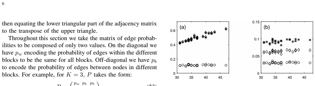
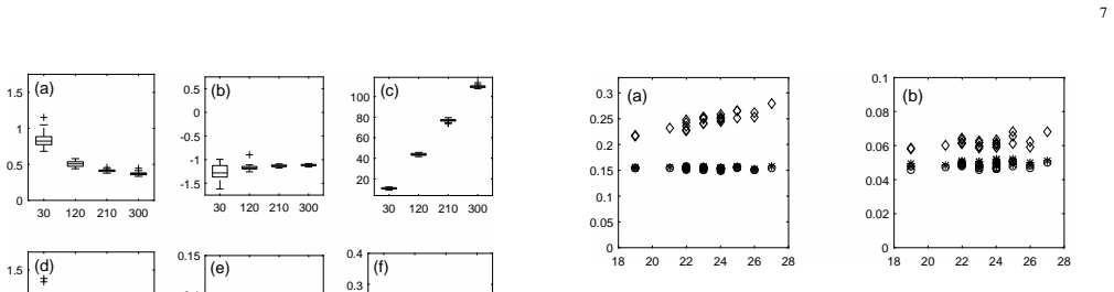
- [Section V-C, Figs. 1 and 2] The examples with j = 1, r = 2 are the ones where the strict-inequality relaxation is most delicate, since Proposition 1's asymptotic guarantee applies only to j = 0 or j = n−r. For the graph-shift-operator comparisons in Section V-C, the authors do not report how often the cvx solution of the relaxed problem satisfied the strict constraints, nor how often the optimum occurred on a boundary, nor what the slack values were. Given that this example is the primary demonstration of cases where the standard Davis–Kahan theorem does not apply, the paper would be substantially strengthened by reporting these diagnostics. Without them, the reader cannot verify that the reported 'bound values' are valid for Theorem 5 of Paper I rather than values of the relaxed objective.
- [Section V-B, Eq. (24)] Equation (24) contains a sign issue that is never addressed. The displayed chain states ||Wj − VjQ||_F ≤ ||WjW_j^T − (I − VjV_j^T)||_2 ≤ ...; the correct projector difference from Eq. (1) is ||WjW_j^T (I − VjV_j^T)||_2, not ||WjW_j^T − (I − VjV_j^T)||_2. These two quantities are not equal in general for r > 1. The text and figures labeled 'ρ2' rely on the correct form in the prose, but Eq. (24) is formally wrong and would confuse any reader attempting to reproduce the metric. This is a presentation error rather than a fatal one, but it should be corrected because Eq. (24) is the displayed definition used throughout the application section.
minor comments (6)
- [Section IV-D] The sentence 'In the original proposal of the transformation for linear fractional programs [4] the equality constraint ||y1Φ + y2I − tΨ||_2 = 1 was used' should specify that for linear fractional programs the equality constraint is an affine equality after the Charnes–Cooper substitution, which is why it is admissible there; the subsequent comparison with convex programs would then be clearer.
- [Section IV-E] In Eq. (22), the variable names are inconsistent: the text introduces the affine transformation parameters (c1,c0), but the displayed Dinkelbach problem uses (c,d). The notation should be unified.
- [Appendix A] The l'Hôpital argument in the appendix computes limits of the lower and upper bounds in (25) and (26), but the sandwich conclusion is stated only in words. A single displayed chain of inequalities for each δ would make the proof easier to check; in particular, it should be explicit that the same c1 is held fixed while c0 tends to ±∞.
- [Section V-C] The text says 'degree extreme differences' but the x-axes of Figs. 1 and 3 are not defined in the captions. The authors should state exactly which quantity is plotted (e.g., max degree minus min degree) and how it is computed for each graph shift operator.
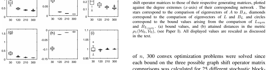
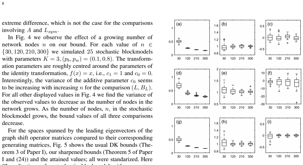
- [Section V-D, Fig. 5] In Fig. 5(b), the text highlights simulation number 10 as a case where the bound is 'very close to tight'; it would be useful to state the numerical values of the attained ρ2 distance and the bound for that simulation, since the figure alone does not allow the reader to verify the claimed proximity.
- [General] There are several typographical issues: in the abstract 'sec ond' appears as 'second' after a line break rendering; in Section V-B the re-scaled expression 'c−1_n,r' is used without defining the scaling of the metrics ρ1 and ρ2; and the references in the introduction are cited in an ad-hoc numeric order (e.g., [9], [13] before [5], [18]). These do not affect the mathematics.
Circularity Check
No circularity: the affine-bound optimization is self-contained conditional on Paper I's theorem, and comparisons use independently attained distances.
full rationale
The paper's derivation chain is: take Paper I's extended Davis–Kahan theorem and Constraints 2, specialize to affine transformations, formulate the ratio ||c1 Phi + c0 I - Psi|| / delta as a fractional program, and compute its global optimum via (15), (19), and (21). None of these steps defines its output in terms of its target: the bound values are computed solely from the transformation parameters and the given spectra through (11)-(14) and (15), while the 'attained distances' to which the bounds are compared are computed independently from the eigenvector spaces (Section V-B, metrics rho1 and rho2, and Figures 1-8). The claim that the affine extended bound is at least as tight as the standard Davis-Kahan bound follows from the identity transformation f(x)=x being feasible whenever the standard theorem applies; this is a valid inclusion-of-feasible-set argument, not a fit or a tautology. The reliance on Theorem 5 of Paper I is a mathematical dependency and a self-citation, but not a circular one: that theorem is parameter-free, its assumptions are stated and do not include the optimization output or the example distances, and this paper does not redefine or assume the result it claims to compute. The strict-inequality relaxation in the cvx implementation (Section IV-D, 'cvx does not accept strict inequalities... then check whether the obtained solutions satisfy the strict inequalities') is a transparency-correctness caveat about boundary optima, not a circularity, because it does not make the computed bound equal to its inputs. Overall, no equation or claim was found in which a predicted bound reduces by construction to a fitted parameter or to an input quantity.
Assumptions & free parameters
assumptions (4)
- domain assumption The extended Davis-Kahan theorem of Paper I (Theorem 5) gives the upper bound (1) for polynomial matrix transformations.
- domain assumption Constraints 2 of Paper I characterize the DK interval separation for affine transforms, giving the formulas for delta in Equations (11) to (14).
- standard math For concave-convex fractional programs, any local maximum is global, and the Charnes-Cooper transformation with the relaxed inequality constraint is equivalent to the original problem.
- domain assumption The stochastic blockmodel and spiked covariance models generate symmetric matrices with the eigenvalue structure the examples rely on.
Cite this review
Pith. "Pith review of Extending the Davis-Kahan theorem for comparing eigenvectors of two symmetric matrices II: Computation and Applications." pith.science (2026). https://pith.science/paper/XH6DGEPV
@misc{pith2026190803465,
  author       = {Pith},
  title        = {Pith review of: Extending the Davis-Kahan theorem for comparing eigenvectors of two symmetric matrices II: Computation and Applications},
  year         = {2026},
  howpublished = {\url{https://pith.science/paper/XH6DGEPV}},
  note         = {Machine review of arXiv:1908.03465}
}
read the original abstract
The extended Davis-Kahan theorem makes use of polynomial matrix transformations to produce bounds at least as tight as the standard Davis-Kahan theorem. The optimization problem of finding transformation parameters resulting in optimal bounds from the extended Davis-Kahan theorem is presented for affine transformations. It is demonstrated how globally optimal bound values can be computed automatically using fractional programming theory. Two different solution approaches, the Charnes-Cooper transformation and Dinkelbach's algorithm are reviewed. Our implementation of the extended Davis--Kahan theorem is used to calculate bound values in three significant examples. First, a pairwise comparison is made of the spaces spanned by the eigenvectors of the graph shift operator matrices corresponding to different stochastic block model graphs. Second our bound is calculated on the distance of the spaces spanned by eigenvectors of the graph shift operators and their corresponding generating matrices in the stochastic blockmodel, and, third, on the sample and population covariance matrices in a spiked covariance model. Our extended bound values, using affine transformations, not only outperform the standard Davis-Kahan bounds in all examples where both theorems apply, but also demonstrate good performance in several cases where the standard Davis-Kahan theorem cannot be used.
Figures
Figures from the paper (4 more)
Reference graph
Works this paper leans on
-
[1]
D. S. Bernstein, Matrix Mathematics: Theory, Facts, and F ormulas (2nd. Edition), Princeton, NJ: Princeton University Press, 2009
2009
- [2]
-
[3]
Signal-plus-noise matri x models: eigenvector deviations and fluctuations,
J. Cape, M. Tang & C. E. Priebe, “Signal-plus-noise matri x models: eigenvector deviations and fluctuations,” Biometrika, vol. 106, pp. 243 – 250, 2019
2019
-
[4]
Programming with linear fract ional functionals,
A. Charnes & W. W. Cooper, “Programming with linear fract ional functionals,” Naval Research logistics quarterly , vol. 9, pp. 181 – 186, 1962
work page 1962
-
[5]
K. T. K. Cheung & L. Hanzo, “Distributed Energy Spectral E fficiency Optimization for Partial/Full Interference Alignment in M ulti-user Multi- relay Multi-cell MIMO Systems,” IEEE Transactions on Signal Pro- cessing, vol. 64, pp. 882–896, 2016
work page 2016
-
[6]
On Nonlinear Fractional Programming,
W. Dinkelbach, “On Nonlinear Fractional Programming,” Management Science, vol. 13, pp. 492–498, 1967
work page 1967
-
[7]
Unperturbed: spectral analysis beyond Davis–Kahan,
J. Eldridge, M. Belkin & Y . Wang, “Unperturbed: spectral analysis beyond Davis–Kahan,” Proceedings of Algorithmic Learning Theory , vol. 83, pp. 321–358, 2018
2018
-
[8]
Large covariance estimati on by thresholding principal orthogonal complements,
J. Fan, Y . Liao & M. Mincheva, “Large covariance estimati on by thresholding principal orthogonal complements,” Journal of the Royal Statistical Society B , vol. 75, pp. 603–680, 2013
2013
Show all 28 references
-
[9]
Frenk & S
H. Frenk & S. Schaible, Fractional Programming, In: C. Floudas , P . Pardalos (eds) Encyclopedia of Optimization, Boston, MA: Springer, 2009. 11
2009
-
[10]
Grant & S
M. Grant & S. Boyd, CVX: Matlab software for disciplined con- vex programming, version 2.1, http://cvxr.com/cvx, Accessed: September 2018
2018
-
[11]
Grant & S
M. Grant & S. Boyd, Graph implementations for nonsmooth convex programs, In: V . Blondel, S. Boyd, H. Kimura (eds) Recent Adv ances in Learning and Control, Boston, MA: Springer, 2008
2008
-
[12]
Stochastic B lockmodels: First Steps,
P . W. Holland, K. B. Laskey & S. Leinhardt, “Stochastic B lockmodels: First Steps,” Social Networks , vol. 5, pp. 109–137, 1983
1983
-
[13]
Frame work for link- level energy efficiency optimization with informed transmi tter,
C. Isheden, Z. Chong, E. Jorswieck & G. Fettweis, “Frame work for link- level energy efficiency optimization with informed transmi tter,” IEEE Transactions on Wireless Communications , vol. 11, pp. 2946–2957, 2012
2012
-
[14]
On the distribution of the largest eig envalue in prin- cipal components analysis,
I. M. Johnstone, “On the distribution of the largest eig envalue in prin- cipal components analysis,” The Annals of Statistics , vol. 29, pp. 295– 327, 2001
2001
-
[15]
PCA consistency in High Dimensio n Low Sample Size Context,
S. Jung & J. S. Marron, “PCA consistency in High Dimensio n Low Sample Size Context,” The Annals of Statistics , vol. 37, pp. 4104–4130, 2009
2009
-
[16]
Stochastic blockmodels and community structure in networks,
B. Karrer & M. E. J. Newman, “Stochastic blockmodels and community structure in networks,” Phys. Rev. E , vol. 83, pp. 016107, 2011
2011
-
[17]
Consistency of spectral clusterin g in stochastic block models,
J. Lei & A. Rinaldo, “Consistency of spectral clusterin g in stochastic block models,” The Annals of Statistics , vol. 43, pp. 215–237, 2015
2015
-
[18]
Fractional QCQP With Applications in ML Steering Direction Estimation for Radar Detection,
A. De Maio, Y . Huang, D. P . Palomar, S. Zhang & A. Farina, “ Fractional QCQP With Applications in ML Steering Direction Estimation for Radar Detection,” IEEE Transactions on Signal Processing , vol. 59, pp. 172– 185, 2011
2011
-
[19]
Spectral clustering and the high- dimensional stochastic blockmodel,
K. Rohe, S. Chatterjee & B. Y u, “Spectral clustering and the high- dimensional stochastic blockmodel,” The Annals of Statistics , vol. 39, pp. 1878–1915, 2011
1915
-
[20]
Parameter-free Convex Equivalent and Du al Programs of Fractional Programming Problems,
S. Schaible, “Parameter-free Convex Equivalent and Du al Programs of Fractional Programming Problems,” Zeitschrift f¨ ur Operations Research, vol. 18, pp. 187–196, 1974
1974
-
[21]
Minimization of Ratios,
S. Schaible, “Minimization of Ratios,” Journal of optimization theory and applications , vol. 19, pp. 347–352, 1976
1976
-
[22]
Fractional Programming: Applications a nd algorithms,
S. Schaible, “Fractional Programming: Applications a nd algorithms,” European Journal of Operations Research , vol. 7, pp. 111–120, 1981
1981
-
[23]
Fractional Programming,
S. Schaible, “Fractional Programming,” Zeitschrift f¨ ur Operations Re- search, vol. 27, pp. 39–54, 1983
1983
-
[24]
A general framework for c onsist- ency of principal component analysis,
D. Shen, H. Shen & J. S. Marron, “A general framework for c onsist- ency of principal component analysis,” Journal of Machine Learning Research, vol. 17, pp. 1–34, 2016
2016
-
[25]
Fractional Programming for Communicat ion Systems—Part I: Power Control and Beamforming,
K. Shen & W. Y u, “Fractional Programming for Communicat ion Systems—Part I: Power Control and Beamforming,” IEEE Transactions on Signal Processing , vol. 66, pp. 2616–2630, 2018
2018
-
[26]
Asymptotics of empirical eigenstruct ure for high dimensional spiked covariance,
W. Wang & J. Fan, “Asymptotics of empirical eigenstruct ure for high dimensional spiked covariance,” The Annals of Statistics , vol. 45, pp. 1342–1374, 2017
2017
-
[27]
Dynamic Asymmetr ic Power Splitting Scheme for SWIPT-Based Two-Way Multiplica tive AF Relaying,
Y . Y e, Y . Li, Z. Wang, X. Chu & H. Zhang, “Dynamic Asymmetr ic Power Splitting Scheme for SWIPT-Based Two-Way Multiplica tive AF Relaying,” IEEE Signal Processing Letters , vol. 25, pp. 1014–1018, 2018
2018
-
[28]
A useful variant of the Da vis–Kahan theorem for statisticians,
Y . Y u, T. Wang & R. J. Samworth, “A useful variant of the Da vis–Kahan theorem for statisticians,” Biometrika, vol. 102, pp. 315–323, 2015
2015
Reviewed August 14, 2026 · model on record in the stance chip above.
Discussion (0). Continue with ORCID to comment.