REVIEW 3 major objections 5 minor 42 references
Hardware-efficient quantum algorithm for the simulation of open-system dynamics and thermalisation
T0 review · 3 major / 5 minor · reviewed 2026-08-14 · deepseek-v4-flash
Pith's one-line read Open-system dynamics simulated with a tiny surrogate environment
desk verdict A clean compression construction for open-system simulation with a real qubit saving; the dissipation protocols are heuristic, so the central claim needs error bounds before it is fully hardened. read the letter →
The pith
A machine-rendered reading of the paper's core claim, the machinery that carries it, and where it could break.
The reading
What carries the argument
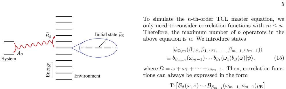
The load-bearing object is the relevant-state set $V_n=\{|\varphi_{\Omega,m}(\cdots)\rangle\}$: states formed by applying up to $\lfloor n/2\rfloor$ transition operators $b_\beta(\omega)$ to the purification $|\psi\rangle$ of the stationary reservoir state. Every $m$-time correlation function with $m\le n$ can be written as an overlap $\langle \varphi_{\Omega_L,m_L}|b|\varphi_{\Omega_R,m_R}\rangle$ with $m_L,m_R\le \lfloor n/2\rfloor$, so all correlation information lives in this subspace. The algorithm computes the Gram matrix $g_{\varphi,\varphi'}=\langle\varphi|\varphi'\rangle$ and the matrix elements $b_{\varphi,\varphi'}=\langle\varphi|b|\varphi'\rangle$ classically, orthonormalises the set, and uses the resulting $d_E$-dimensional representation to define the surrogate environment: $\tilde\rho_E=|\tilde\psi\rangle\langle\tilde\psi|$, $\tilde H_E=-\sum_\Omega \Omega\,\tilde\Pi_\Omega$, and $\tilde B_\beta=\sum_\omega \tilde b_\beta(\omega)$. Theorem 1 is the criterion that makes this representation sufficient for the time-convolutionless expansion.
What would settle it
Choose a concrete bath, such as the Lorentzian spectral density of Sec. IX, compute its two- and four-time correlation functions numerically, construct the surrogate with dimension $d_E$, and test whether $\langle \tilde B_{\beta}(t)\cdots\tilde\rho_E\rangle$ matches the original correlation functions for all $m\le n$ beyond the spectrum-discretisation error; any mismatch would refute the sufficiency claim of Theorem 1. A sharper probe is to evolve the surrogate under the fourth-order TCL generator and verify that the conditional dissipation protocol reduces $\tilde K_4(t)$ to $O(\tau_E^3)$ rather than leaving $O(\tau_E^2 t)$.
Extended reading notes
Core claim
The central claim is Theorem 1: two environments coupled to the same system through the same system operators $A_\beta$ induce identical system dynamics up to order $n$ whenever all their reservoir correlation functions of orders $m\le n$ agree. The paper then shows how to build the smallest such surrogate. Purify the stationary environment state $\rho_E$ to $|\psi\rangle$, and for each frequency $\omega$ and coupling index $\beta$ define $b_\beta(\omega)=B_\beta(\omega)\otimes 1_a$ acting on the purification. The states $|\varphi_{\Omega,m}(\cdots)\rangle=b_{\beta_{m-1}}(\omega_{m-1})\cdots b_{\beta}(\omega)|\psi\rangle$ with $m\le \lfloor n/2\rfloor$ span a relevant-state space of dimension at most $d_{n,\max}=[(N_\omega N_\beta)^{\lfloor n/2\rfloor+1}-1]/[N_\omega N_\beta-1]$, so roughly $\lfloor n/2\rfloor \log_2(N_\omega N_\beta)$ qubits represent the environment. A classical Gram-Schmidt step converts the Gram matrix and operator overlaps of this set into an explicit $d_E$-dimensional Hamiltonian $\tilde H_E$ and interaction operators $\tilde B_\beta$; Theorem 1 then guarantees that the small environment reproduces the correct reduced dynamics up to order $n$, with long-time evolution handled by reinitialising or dissipating the small environment without significantly changing the correlation functions.
Load-bearing premise
The load-bearing premise is the paper's explicit assumption that reservoir correlation functions of the original environment are computable in classical computation: if those functions (or the Gram matrix built from them) are not classically available, the small surrogate environment cannot be designed and the qubit saving disappears.
Editorial extensions
If this is right
- The $n$-th-order TCL master equation can be simulated with an environment of roughly $\lfloor n/2\rfloor \log_2(N_\omega N_\beta)$ qubits, so for $n=2$ the environment can be much smaller than the system.
- Markovian master equations and thermalisation, including zero-temperature ground-state preparation, become accessible with a small number of environment qubits whenever the reservoir correlation functions are classically computable.
- Non-Markovian dynamics can be reached by increasing $n$, with an environment size that grows only logarithmically in $N_\omega N_\beta$ and linearly in $n$.
- The Trotterised circuit has gate count $O(N_E N_\omega^{2n} N_\beta^{2n+2})$, so the qubit saving comes with a polynomial overhead in the spectral and coupling parameters.
- Periodic reinitialisation or conditional dissipation of the small environment suppresses the finite-size fourth-order error from $O(\tau_E^2 t)$ to $O(\tau_E^3)$, restoring long-time thermalisation behaviour.
Reading between the lines
- Because the construction only needs the Gram matrix of $V_n$, a surrogate environment could in principle be built from experimentally measured correlation functions instead of a known Hamiltonian, extending the method to baths whose microscopic model is unavailable.
- The dimension bound $d_{n,\max}\approx (N_\omega N_\beta)^{\lfloor n/2\rfloor}$ suggests a connection to tensor-network and matrix-product representations of bath correlation functions: the Gram matrix rank characterises when a spectral density admits a small exact environment.
- If the classical-computability assumption fails, the same relevant-state construction could be run in reverse, using a quantum computer to prepare the states $|\varphi\rangle$ and estimate the Gram matrix statistically, at the price of replacing exact design with certified sampling.
- For thermalisation, the algorithm offers a route to ground-state preparation that avoids diagonalising the system Hamiltonian; this is an implicit consequence of the paper's construction rather than a result the authors emphasise.
Signed reviews
Editorial analysis
A structured set of objections, weighed in public.
Referee Report
Summary. The paper proposes a quantum algorithm for simulating open-system dynamics by replacing the physical environment with a compressed one that reproduces the reservoir correlation functions up to a chosen order n. The main theoretical result (Theorem 1, Sec. II) states that matching all m-time correlation functions for m≤n is sufficient for the system dynamics to agree with the n-th-order time-convolutionless (TCL) expansion. Sections IV-VI construct such an environment from the Gram matrix of the relevant state set V_n, bounding its dimension by d_n,max=(NωNβ)^floor(n/2); for n=2 this reduces to a small environment reproducing two-time correlations and hence, under the Markov approximation, the Markovian master equation. Section VII introduces dissipation protocols to relax the finite environment, Sec. VIII gives qubit and gate-count estimates, and Sec. IX presents a classical simulation of qubit thermalisation at zero and finite temperature.
Significance. If the construction of Secs. IV-VI and Theorem 1 are correct, the paper contributes a conceptually clean dimension-reduction argument: matching reservoir correlation functions up to order n suffices for the n-th-order TCL dynamics, and the environment can be compressed to roughly floor(n/2) log2(NωNβ) qubits. The Gram-Schmidt construction in Appendix A and the norm bound in Appendix C are explicit and checkable, and the n=2 case gives a concrete small-environment route to Markovian master-equation simulation. However, as detailed in the major comments, the error analysis for the dissipative protocols and the accounting of the classical precomputation cost are missing, so the end-to-end claim of hardware-efficient simulation of thermalisation is not yet fully established.
major comments (3)
- [Sec. VII, esp. VII B/VII C, and Theorem 1 in Sec. II/VI] The equivalence proved in Theorem 1 and Appendix B applies to the bare Hamiltonian dynamics with a stationary environment and no additional dissipation. The protocols introduced to suppress finite-size effects modify the very correlation functions on which the construction is based: in the projective protocol Eq. (23) gives V_i = e^{-Γ s_i} 11 + (1-e^{-Γ s_i})P, so two-time functions acquire a factor e^{-Γ(t-s)}; in the conditional protocol the claim that correlation functions are only slightly modified is asserted from localization assumptions (the wave-packet argument of Sec. VII C) rather than proven. Consequently the manuscript does not bound ||ρ_S^sim(t) - ρ_S^TCL(t)|| for the algorithm actually executed on the quantum computer; the estimates such as ~K4(t)=O(τ_E^2 Γ^{-1}) or O(τ_E^3) are heuristic scalings, not error bounds. This gap is load-bearing because the central claim, that the small environment plus dissipation simulates the Markovian master equation and thermalisation, concerns the dissipative protocol rather than the bare Hamiltonian construction alone.
- [Sec. VI A and Appendix A; Sec. III assumption; Sec. VIII resource count] The resource estimate in Sec. VIII counts only the qubit number N_E and gate count N_G. The classical precomputation is not counted: for an n-th-order simulation one must form the Gram matrix of the set V_n, whose size is d_n,max=(NωNβ)^floor(n/2), and perform Gram-Schmidt orthogonalisation; even the most favorable accounting is at least O(d_n,max^2) to build the Gram matrix and at least O(d_n,max d_E^2) for the orthogonalisation, and a direct matrix-inversion view costs O(d_n,max^3). For the illustrative parameters in Sec. VIII, Nω=10^6, Nβ=10^3, n=2, this is already a 10^9×10^9 matrix problem. Since Sec. III explicitly assumes the correlation functions are classically computable, the additional cost of this construction must be stated and bounded before the 'hardware-efficient' claim is complete; otherwise the algorithm is end-to-end efficient only under a further unstated assumption.
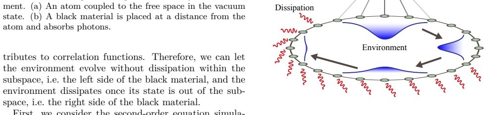
- [Sec. IX, Fig. 6] The numerical validation of thermalisation at finite temperature does not provide a parameter-free confirmation of the algorithm. The Fig. 6 caption explicitly states that the dissipation zone 3≤x≤398 was 'chosen to obtain the best fit to the Lindblad equation.' Thus the good agreement between the red circles and the black Lindblad curve in Fig. 6 is partly the result of fitting the simulation to the target curve. To support the claim that the protocol simulates thermalisation without prior knowledge of the Lindblad equation, the dissipation parameters should be fixed a priori from the correlation-time and wave-packet arguments of Sec. VII C, with a robustness check over a range of dissipation-zone positions, or the fit should be clearly presented only as an illustration of the protocol's tuning flexibility.
minor comments (5)
- [Sec. VIII] The phrase 'Trotterisation algoirthm' contains a typo; it should read 'Trotterisation algorithm'.
- [References] Reference [3] is cited as 'Rev. Mod. Phys. A 89, 015001 (2017)' but should be 'Rev. Mod. Phys. 89, 015001 (2017)'; reference [41] is cited as 'Mo. Phys.' and should be 'Mol. Phys.'.
- [Eq. (5)] The notation in Eq. (5) is very dense; an explicit example for m=2, showing how κ2 reduces to an integral over two-time correlation functions in the form of Eq. (7), would substantially improve readability and help the reader connect the superoperator formalism to the intuitive correlation-function condition.
- [Sec. VII A and VII B] Equation (23) is reused for both the periodic reinitialisation protocol and the projective dissipation protocol, but the meaning of V_i is different in the two cases: a projection P in the former and the mixture e^{-Γ s_i} 11 + (1-e^{-Γ s_i})P in the latter. Please separate the two definitions to avoid confusion.
- [Sec. VII C] The statement that 'the propagation from |x⟩ to |x+1⟩ takes the time c^{-1}' would benefit from an explicit derivation from Eqs. (24)-(25) and the definition c = Nωδω/(2π); as written, the speed of the wave-package in the x-representation is stated rather than shown.
Circularity Check
Core construction is self-contained; only the finite-temperature numerical validation fits a dissipation-zone parameter to the Lindblad target.
-
fitted input called prediction
[Section IX, Fig. 6 caption]
"The dissipation zone is 3 ≤ x ≤ 398 for the finite temperature, which is chosen to obtain the best fit to the Lindblad equation of the thermalisation."
In the illustrative validation, a parameter of the simulated environment (the conditional-reinitialisation dissipation zone) is explicitly tuned to make the finite-temperature simulation best match the target Lindblad thermalisation curve. The displayed agreement between the simulated pg(t) and the Lindblad curve is therefore partly by construction and does not serve as a parameter-free test of the algorithm. This is a local validation blemish only: the construction in Secs. IV–VI is parameter-free given the classically supplied reservoir correlation functions, and the central derivation does not depend on this fitted zone.
full rationale
The central derivation is not circular. The paper takes reservoir correlation functions as externally supplied inputs, constructs a d_E-dimensional representation of the relevant state space from the Gram matrix, and proves in Appendix B (via Eq. (17)) that the constructed environment reproduces the same correlation functions up to the chosen TCL order. Theorem 1 is then used to infer equal dynamics from equal correlation functions; it is proved in the paper from the TCL expansion, not imported from a self-citation or asserted by definition. There are no load-bearing self-citations: the only co-author citations (e.g. Refs. [36,37]) are for variational/imaginary-time methods and are not used as the correctness certificate. The stated assumption that correlation functions are classically computable (Sec. III) is an input assumption, not a circular step. The conditional-dissipation argument in Sec. VII C relies on localization assumptions and heuristic order estimates rather than a rigorous distance bound, but that is a completeness/correctness gap, not circularity. The only concrete circular element is the finite-temperature validation in Fig. 6, where the dissipation zone is explicitly chosen to best fit the Lindblad curve, making that comparison partly a fit. This does not infect the algorithm itself, so the overall circularity score is low.
Assumptions & free parameters
free parameters (2)
- Finite-temperature dissipation zone bounds =
3 <= x <= 398
- Zero-temperature dissipation zone bounds =
21 <= x <= 380
assumptions (7)
- domain assumption The environment state rhoE is stationary, [HE, rhoE] = 0, and interaction operators satisfy Tr(Bbeta rhoE) = 0 after absorbing the mean field into HS.
- domain assumption Reservoir correlation functions of the original environment are classically computable, including the Gram matrix of states V_n.
- domain assumption Truncating the TCL expansion at order n gives an adequate approximation of the open-system dynamics.
- domain assumption For thermalisation simulation, the Markov approximation K2(t) approximately K2(infinity) and weak coupling are valid.
- domain assumption The environment spectrum can be discretised with Nomega frequencies such that correlation functions converge polynomially and the recurrence time exceeds the simulation time.
- domain assumption For conditional dissipation, the system-environment coupling is local in the x representation, so wavepackets are confined to 0 <= x <= xE.
- standard math Standard linear algebra: purification with rank(rhoE) ancillary dimensions, Gram-Schmidt orthonormalisation, and the cyclic property of trace.
Cite this review
Pith. "Pith review of Hardware-efficient quantum algorithm for the simulation of open-system dynamics and thermalisation." pith.science (2026). https://pith.science/paper/QA7R5BF6
@misc{pith2026190803759,
  author       = {Pith},
  title        = {Pith review of: Hardware-efficient quantum algorithm for the simulation of open-system dynamics and thermalisation},
  year         = {2026},
  howpublished = {\url{https://pith.science/paper/QA7R5BF6}},
  note         = {Machine review of arXiv:1908.03759}
}
abstract
The quantum open-system simulation is an important category of quantum simulation. By simulating the thermalisation process at the zero temperature, we can solve the ground-state problem of quantum systems. To realise the open-system evolution on the quantum computer, we need to encode the environment using qubits. However, usually the environment is much larger than the system, i.e. numerous qubits are required if the environment is directly encoded. In this paper, we propose a way to simulate open-system dynamics by reproducing reservoir correlation functions using a minimised Hilbert space. In this way, we only need a small number of qubits to represent the environment. To simulate the $n$-th-order expansion of the time-convolutionless master equation by reproducing up to $n$-time correlation functions, the number of qubits representing the environment is $\sim \lfloor \frac{n}{2} \rfloor \log_2(N_\omega N_\beta)$. Here, $N_\omega$ is the number of frequencies in the discretised environment spectrum, and $N_\beta$ is the number of terms in the system-environment interaction. By reproducing two-time correlation functions, i.e. taking $n = 2$, we can simulate the Markovian quantum master equation. In our algorithm, the environment on the quantum computer could be even smaller than the system.
Figures


Figures from the paper (3 more)


Reference graph
Works this paper leans on
-
[38]
I. A. Luchnikov, S. V. Vintskevich, H. Ouerdane, and S. N. Filippov, Simulation complexity of open quantum dynamics: Connection with tensor networks , Phys. Rev. Lett. 122, 160401 (2019)
work page 2019
-
[1]
Feynman, Simulating physics with computers , Int
R. Feynman, Simulating physics with computers , Int. J. Theor. Phys. 21, 467 (1982)
work page 1982
-
[2]
H.-P. Breuer and F. Petruccione, The Theory of Open Quantum Systems, Oxford University Press, (2007)
work page 2007
-
[3]
I. de Vega and D. Alonso, Dynamics of non-Markovian open quantum systems , Rev. Mod. Phys. A 89, 015001 (2017)
work page 2017
-
[4]
Lloyd, Universal quantum simulators , Science 273, 1073 (1996)
S. Lloyd, Universal quantum simulators , Science 273, 1073 (1996)
1996
-
[5]
B. M. Terhal and D. P. DiVincenzo, Problem of equili- bration and the computation of correlation functions on a quantum computer , Phys. Rev. A 61, 022301 (2000)
work page 2000
-
[6]
H. Wang, S. Ashhab, and F. Nori, Quantum algorithm for simulating the dynamics of an open quantum system , Phys. Rev. A 83, 062317 (2011)
work page 2011
-
[7]
D. Abrams and S. Lloyd, Quantum algorithm provid- ing exponential speed increase for finding eigenvalues and eigenvectors, Phys. Rev. Lett. 83, 5162 (1999)
work page 1999
Show all 42 references
-
[8]
Aspuru-Guzik, A
A. Aspuru-Guzik, A. D. Dutoi, P. J. Love, and M. Head- Gordon, Simulated Quantum Computation of Molecular Energies, Science 309, 1704 (2005)
2005
-
[9]
Wecker, B
D. Wecker, B. Bauer, B. K. Clark, M. B. Hastings, and M. Troyer, Gate-count estimates for performing quantum chemistry on small quantum computers, Phys. Rev. A90, 022305 (2014)
2014
-
[10]
Bauer, D
B. Bauer, D. Wecker, A. J. Millis, M. B. Hastings, and M. Troyer, Hybrid quantum-classical approach to correlated materials, Phys. Rev. X 6, 031045 (2016)
2016
-
[11]
Verstraete, M
F. Verstraete, M. M. Wolf, and J. I. Cirac,Quantum com- putation and quantum-state engineering driven by dissi- pation, Nature Phys. 5, 633 (2009)
2009
-
[12]
Farhi, J
E. Farhi, J. Goldstone, S. Gutmann, J. Lapan, A. Lund- gren, and D. Preda, A quantum adiabatic evolution al- gorithm applied to random instances of an NP-complete problem, Science 292, 472 (2001)
2001
-
[13]
A. Y. Kitaev, A. H. Shen and M. N. Vyalyi, Classical and quantum computation, American Mathematical Society, (2002)
2002
- [14]
-
[15]
Poulin and P
D. Poulin and P. Wocjan Sampling from the thermal quantum Gibbs state and evaluating partition functions with a quantum computer , Phys. Rev. Lett. 103, 220502 (2009)
2009
-
[16]
Bilgin and S
E. Bilgin and S. Boixo, Preparing thermal states of quan- tum systems by dimension reduction , Phys. Rev. Lett. 105, 170405 (2010)
2010
-
[17]
Temme, T
K. Temme, T. J. Osborne, K. G. Vollbrecht, D. Poulin, and F. Verstraete, Quantum Metropolis sampling, Nature 471, 87 (2011)
2011
-
[18]
Riera, C
A. Riera, C. Gogolin, and J. Eisert, Thermalization in nature and on a quantum computer , Phys. Rev. Lett. 108, 080402 (2012)
2012
-
[19]
Yung and A
M.-H. Yung and A. Aspuru-Guzik, A quantum-quantum Metropolis algorithm, PNAS 109, 754 (2012)
2012
-
[20]
Motta, C
M. Motta, C. Sun, A. T. K. Tan, M. J. O’Rourke, E. Ye, A. J. Minnich, F. G. S. L. Brandao, and G. Kin-Lic Chan, Quantum imaginary time evolution, quantum lanczos, and quantum thermal averaging , arXiv:1901.07653
1901 arXiv
-
[21]
Campbell, Random compiler for fast Hamiltonian sim- ulation, Phys
E. Campbell, Random compiler for fast Hamiltonian sim- ulation, Phys. Rev. Lett. 123, 070503 (2019)
2019
-
[22]
D. W. Berry, G. Ahokas, R. Cleve, B. C. Sanders, Effi- cient quantum algorithms for simulating sparse Hamilto- nians, Commun. Math. Phys. 270, 359 (2007)
2007
-
[23]
Wiebe, D
N. Wiebe, D. Berry, P. Høyer, and B. C. Sanders, Higher order decompositions of ordered operator exponentials, J. Phys. A: Math. Theor. 43, 065203 (2010)
2010
-
[24]
D. W. Berry, A. M. Childs, R. Cleve, R. Kothari, and R. D. Somma, Simulating Hamiltonian dynamics with a truncated Taylor series , Phys. Rev. Lett. 114, 090502 (2015). 14
2015
-
[25]
Bacon, A
D. Bacon, A. M. Childs, I. L. Chuang, J. Kempe, D. W. Leung, and X. Zhou, Universal simulation of Markovian quantum dynamics, Phys. Rev. A 64, 062302 (2001)
2001
-
[26]
Kliesch, T
M. Kliesch, T. Barthel, C. Gogolin, M. Kastoryano, and J. Eisert, Dissipative quantum Church-Turing theorem , Phys. Rev. Lett. 107, 120501 (2011)
2011
-
[27]
Sweke, I
R. Sweke, I. Sinayskiy, D. Bernard, and F. Petruccione, Universal simulation of Markovian open quantum sys- tems, Phys. Rev. A 91, 062308 (2015)
2015
-
[28]
Di Candia, J
R. Di Candia, J. S. Pedernales, A. del Campo, E. Solano, and J. Casanova, Quantum simulation of dissipative pro- cesses without reservoir engineering , Sci. Rep. 5, 9981 (2015)
2015
-
[29]
Sweke, M
R. Sweke, M. Sanz, I. Sinayskiy, F. Petruccione, and E. Solano, Digital quantum simulation of many-body non- Markovian dynamics, Phys. Rev. A 94, 022317 (2016)
2016
-
[30]
A. M. Childs and T. Li, Efficient simulation of sparse Markovian quantum dynamics , QIC 17, 901 (2017)
2017
-
[31]
Chenu, M
A. Chenu, M. Beau, J. Cao, and A. del Campo, Quantum simulation of generic many-body open system dynam- ics using classical noise , Phys. Rev. Lett. 118, 140403 (2017)
2017
-
[32]
A. G. Fowler, M. Mariantoni, J. M. Martinis, and A. N. Cleland, Surface codes: Towards practical large-scale quantum computation, Phys. Rev. A 86, 032324 (2012)
2012
-
[33]
O’Gorman and E
J. O’Gorman and E. T. Campbell, Quantum computa- tion with realistic magic state factories , Phys. Rev. A 95, 032338 (2017)
2017
-
[34]
Peruzzo, J
A. Peruzzo, J. McClean, P. Shadbolt, M.-H. Yung, X.-Q. Zhou, P. J. Love, A. Aspuru-Guzik, and J. L. O’Brien, A variational eigenvalue solver on a photonic quantum processor, Nat. Commun. 5, 4213 (2014)
2014
-
[35]
Wecker, M
D. Wecker, M. B. Hastings, and M. Troyer, Progress towards practical quantum variational algorithms , Phys. Rev. A 92, 042303 (2015)
2015
-
[36]
Li and S
Y. Li and S. C. Benjamin, Efficient variational quantum simulator incorporating active error minimisation , Phys. Rev. X 7, 021050 (2017)
2017
-
[37]
McArdle, T
S. McArdle, T. Jones, S. Endo, Y. Li, S. Benjamin, and X. Yuan, Variational quantum simulation of imaginary time evolution, arXiv:1804.03023
-
[39]
Gardiner and P
C. Gardiner and P. Zoller, Quantum noise: A handbook of markovian and non-markovian stochastic process with applications to quantum optics , Springer (2000)
2000
-
[40]
Carmichael, Quantum trajectory theory for cascaded open systems, Phys
H. Carmichael, Quantum trajectory theory for cascaded open systems, Phys. Rev. Lett. 70, 2273 (1993)
1993
-
[41]
J. D. Whitfield, J. Biamonte, and A. Aspuru-Guzik, Sim- ulation of electronic structure Hamiltonians using quan- tum computers, Mo. Phys. 109, 735 (2011)
2011
-
[42]
Ritschel and A
G. Ritschel and A. Eisfeld, Analytic representations of bath correlation functions for ohmic and superohmic spec- tral densities using simple poles , J. Chem. Phys. 141, 094101 (2014)
2014
Reviewed August 14, 2026 · model on record in the stance chip above.
Discussion (0). Continue with ORCID to comment.