Data-Driven Randomized Learning of Feedforward Neural Networks

Grzegorz Dudek

REVIEW 3 major objections 5 minor 9 references

Data-Driven Randomized Learning of Feedforward Neural Networks

T0 review · 3 major / 5 minor · reviewed 2026-08-14 · deepseek-v4-flash

Challenge this review Re-run · record.json Download PDF Read on arXiv ↗ Review JSON

Pith's one-line read A randomized single-hidden-layer network can approximate complex functions by placing each sigmoid at a random training point and setting its weight to four times the local slope fitted to that point's nearest neighbors.

desk verdict A simple, plausible local-slope trick for randomized FNNs, undermined by a reproducibility gap in its headline Kin8nm result. read the letter →

arxiv 1908.03891 v1 pith:Z76DOCDK submitted 2019-08-11 cs.LG cs.NEstat.ML

Grzegorz Dudek This is my paper · ORCID

classification cs.LGcs.NEstat.ML

keywords data-drivenrandomizedlearningfeedforwardneuralnetworkswithrandomhiddennodesalgorithmssigmoidslopeadjustmentlocalhyperplanefittingknearestneighborsregressionapproximation

verification ladder T0 review T1 audit T2 compute T3 formal

The pith

A machine-rendered reading of the paper's core claim, the machinery that carries it, and where it could break.

The reading

This paper proposes a data-driven rule for generating the hidden-neuron parameters of a randomized feedforward network: pick a training point at random, fit a hyperplane to it and its $k$ nearest neighbors, then set the sigmoid weights to four times the hyperplane slopes and the bias so the sigmoid's inflection point sits at the chosen point. The claim is that this places sigmoids where the target function changes and gives each one the local slope of the data, so a linear combination of such sigmoids can approximate strongly nonlinear functions much better than parameters drawn from a fixed interval. On a noisy two-variable target function and on two regression benchmarks, the proposed D-DM method reaches lower test RMSE than the fixed-interval, optimized-interval, and two recent slope-adapting methods, often with fewer hidden nodes. If correct, randomized hidden layers no longer need a hand-tuned parameter interval because their basis functions are locally fitted to the data.

What carries the argument

The load-bearing object is the local hyperplane fit to a random training point's $k$-nearest-neighbor neighborhood, together with the derivative-matching identity $a_j = 4a'_j$. For a logistic sigmoid $h(\mathbf{x}) = (1+\exp(-(\mathbf{a}^\top \mathbf{x}+b)))^{-1}$, the derivative at the inflection point in direction $j$ is $a_j h(1-h)=a_j/4$, so multiplying a fitted slope $a'_j$ by four makes the sigmoid's local directional slope equal the target's local slope as estimated by the hyperplane. The bias formula $b = -\mathbf{a}^\top \mathbf{x}_*$ then anchors each sigmoid's most sensitive part at a real data point. This turns the randomized hidden layer from a random projection into an ensemble of locally tangent basis functions while keeping the output layer a linear least-squares problem.

What would settle it

Compare D-DM and RARSM on the synthetic function $g(x_1,x_2)=\sin(20\exp(x_1))x_1^2+\sin(20\exp(x_2))x_2^2$ with noise $c=0.2$ at the same number of hidden nodes, say $m=300$; if D-DM's test RMSE is not below RARSM's, the claim that local slope matching gives an advantage at matched capacity fails. A more direct check is to compare the hyperplane coefficients used by D-DM with the true partial derivatives of the target at the same anchors: the coefficients should approximate those derivatives after the factor 4.

Watch

Extended reading notes

Core claim

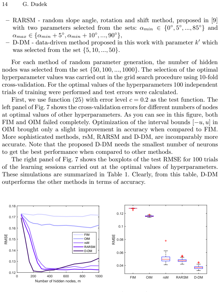
For each hidden node, D-DM draws one training sample $\mathbf{x}_*$, collects the $k$ nearest neighboring training points, and fits a hyperplane $y = a'_1 x_1 + \cdots + a'_n x_n + b'$ to this neighborhood. Because a sigmoid's slope at its inflection point is a quarter of its weight, setting $a_j = 4a'_j$ makes the sigmoid's directional slopes match the hyperplane's local estimates of the target slope; the bias $b = -\mathbf{a}^\top \mathbf{x}_*$ fixes the inflection point exactly at $\mathbf{x}_*$. The fitted curve is then the usual linear combination of these sigmoids with output weights from the pseudoinverse. The paper's key numerical finding is that this construction approximates strongly nonlinear targets with lower RMSE than the baselines: on the Kin8nm benchmark the D-DM test RMSE is 0.0523 versus 0.0618 for the best slope-angle baseline, and on the synthetic function it uses 300 nodes versus RARSM's 350 at a lower error. The intended upshot is that data-anchored, locally scaled sigmoids form a better projection space for randomized networks than interval-sampled parameters.

Load-bearing premise

The whole construction rests on the assumption that the hyperplane fitted to a random training point and its $k$ nearest neighbors gives trustworthy estimates of the target function's local slopes in every input direction; if noise or high dimensionality makes these slope estimates unreliable, the sigmoids are placed with wrong slopes and the advantage over interval-tuned baselines shrinks.

Editorial extensions

If this is right

Strongly nonlinear regression targets can be approximated accurately without searching for a good weight interval; $k$ and the number of hidden nodes $m$ are the only tunable hyperparameters.
Fewer hidden nodes are needed: on the synthetic function D-DM reaches lower RMSE with 300 nodes than RARSM's 350, and on Kin8nm with 900 nodes versus RARSM's 1300.
The hidden layer can be built in one pass plus $k$-nearest-neighbor searches, and the output weights come from the Moore-Penrose pseudoinverse, so no gradient computation enters the learning loop.
The neighborhood size $k$ controls the bias-variance tradeoff: low-noise data favors small neighborhoods ($k'=20$) and high-noise data favors larger ones ($k'=30$), giving a concrete tuning path.

Reading between the lines

Editorial extensions of the paper, not claims the author makes directly.

The same derivative-matching recipe could be extended to other locally fitted basis families, such as radial basis functions centered at random data points, where the local scale would be set by nearest-neighbor distances instead of hyperplane slopes.
In high-dimensional inputs, $k$-nearest-neighbor neighborhoods become less local, so the local hyperplane slope estimates would degrade; a testable fix is to fit hyperplanes in random low-dimensional projections and combine the resulting coordinates.
For classification, anchors chosen near decision-boundary training points rather than uniformly at random should concentrate nonlinear flexibility where class boundaries curve; the paper only demonstrates regression.
If local slope estimates are unstable, averaging hyperplanes over several random anchors per hidden node, or ridge-regressing the neighborhood, might recover accuracy; this is an observable modification of Algorithm 1.

Share X Bluesky LinkedIn Reddit HN

Signed reviews

No signed human review yet.

Editorial analysis

A structured set of objections, weighed in public.

Desk editor's note, referee report, and a circularity audit.

Desk Editor's Note

read the letter

The short version: this is a sensible incremental advance on the author's earlier rsM/RARSM work, and the core derivation is correct. But the strongest real-data result (Kin8nm) is reported with k'=60, outside the D-DM search grid the paper itself specifies, and the grid contains values that Algorithm 1 rules out. That needs fixing before I'd trust the headline numbers.

What's actually new: instead of drawing sigmoid slopes from a global interval, D-DM picks a random training point, fits a hyperplane to its k nearest neighbors, and sets the neuron weights to 4 times the hyperplane slopes, with the bias placing the inflection point at that training point. The sigmoid derivative identity (a/4 at the inflection point) is correct, and the idea of per-neuron slope adaptation to local target curvature is a genuine departure from the earlier interval-based schemes. On the synthetic function and on Stock/Kin8nm, D-DM beats FIM, OIM, rsM, and RARSM, and it uses fewer hidden nodes on the synthetic example. That is a real, if modest, contribution. The paper also clearly explains the bias-variance tradeoff via the neighborhood size k.

The soft spots. First, the protocol mismatch: Section 4 fixes the D-DM k' grid at {5,10,...,50}, but Table 1 shows k'=60 for Kin8nm. For Stock (n=9) and Kin8nm (n=8), the grid values include k'=5, which corresponds to k=4, below the k>=n requirement in Algorithm 1. So the stated hyperparameter search is internally inconsistent, and the one dataset where D-DM shows a decisive improvement is exactly the one whose reported optimum lies outside the declared grid. The authors need to explain whether k'=60 was actually used, and if so, why it is not in the search set; if it is a typo, the real optimum should be reported. Without that, the Kin8nm claim is not reproducible as written.

Second, the evaluation is thin: one synthetic 2-D function and two real datasets, one of which (Stock) shows only a marginal improvement. There is no code, no sensitivity analysis for k on the real data, and no discussion of behavior when the local linearity assumption is violated (e.g., high-dimensional or noisy inputs). These are moderate issues, not fatal. The derivation and the method are sound; the evidence base just needs to be larger and cleaner.

Bottom line: this deserves a serious referee, but it needs a corrected protocol and a broader empirical test. I would conditionally accept if the authors fix the inconsistency and supply code. If you want, I can dig into the equations with you.

Referee Report

3 major / 5 minor

Summary. The paper proposes a data-driven method for generating hidden-node weights and biases in single-hidden-layer feedforward neural networks trained by randomized learning. For each hidden neuron, the method randomly selects a training point, finds its k nearest neighbors, fits a hyperplane to that neighborhood, and sets the sigmoid weights to a_j = 4 a'_j and the bias to b = -a^T x^* (Eqs. 19-24). The output weights are then obtained by least squares. The paper argues that this local slope adjustment places sigmoids so that their steep fragments match local target-function fluctuations, improving approximation accuracy compared with fixed-interval random parameters and earlier interval- or angle-tuned methods. Experiments are reported on one synthetic two-variable function and two real datasets (Stock and Kin8nm).

Significance. If the reported results are reproducible, the method is a simple and potentially useful contribution to randomized neural-network learning. The derivation of a = 4a' from the sigmoid derivative (Eqs. 14-17 and 20-23) is correct, and the algorithm is clearly specified. The idea of adjusting random hidden-node parameters to local data geometry is intuitive and goes beyond the usual fixed-interval generation. The paper also provides extensive simulations with 100 trials and 10-fold cross-validation, which is a reasonable experimental protocol. The main limitation is that the empirical support for the headline claim rests on one synthetic function and two real datasets, one of which (Stock) shows only a marginal improvement over the best baseline; the strongest real-data result (Kin8nm) is currently affected by a reporting inconsistency in the hyperparameter grid, as detailed below. The contribution is significant conditional on correcting that inconsistency.

major comments (3)

[Section 4 vs. Table 1] The declared D-DM neighborhood-size grid is k' in {5, 10, ..., 50}, but Table 1 reports k' = 60 for Kin8nm. This is outside the declared search space. Since the Kin8nm result is the strongest evidence for D-DM (0.0523 vs. 0.0618 for RARSM), the headline comparison is not reproducible as written. Please clarify whether k' = 60 was actually used (and correct the grid description) or rerun the experiment with k' restricted to the declared grid. Additionally, the declared grid contains k' = 5 for Stock (n = 9) and Kin8nm (n = 8), but Algorithm 1 requires k >= n, i.e., k' = k + 1 >= n + 1; those grid points are infeasible and should be removed or the feasibility condition should be restated.
[Table 1, Kin8nm rows] The hidden-node candidate set in Section 4 is declared as {50, 100, ..., 1000}, but Table 1 reports #nodes = 1300 for FIM, OIM, rsM, and RARSM on Kin8nm. This is outside the declared search space, so the comparison protocol is not consistently described. The authors should correct the grid description or the table and confirm that all methods were optimized under the same rules; otherwise the baseline results are not reproducible.
[Section 5 / Abstract] The abstract and conclusions claim that the method 'brings very good results' compared with other methods, but the empirical support is limited to one synthetic function and two real datasets, and on Stock the D-DM improvement over RARSM is small (0.0277 vs. 0.0285 with overlapping standard deviations). If the Kin8nm result is corrected, the strength of the general claim should be moderated, or additional datasets should be added to support the claimed advantage.

minor comments (5)

[Section 3 (intro paragraph)] The text states that 'the weights and biases of the sigmoids are no longer random' (page 7), which is in tension with the paper's use of the term 'randomized learning' and with the abstract's wording about 'random parameters.' Please clarify the terminology: the hidden parameters are data-dependent in this method, not drawn from a fixed distribution, and this departure from the standard randomized-learning setting should be made explicit.
[Section 4] No preprocessing is described for the Stock and Kin8nm datasets. Since the method uses k-nearest-neighbor searches and hyperplane fits, both of which are sensitive to input scaling, the paper should report whether and how the input variables were standardized or normalized.
[Section 4] The notation for the noise bound c in the synthetic experiments conflicts with the random sign variable c in Eq. (10). Please use distinct symbols to avoid confusion.
[Figures 5-6 and text] There is a typo in Fig. 6's y-axis label ('RSME' instead of 'RMSE'), and in the Stock dataset description 'aproximate' should be 'approximate.' These should be corrected in the final version.
[References] Reference [9] is cited as 'in print'; if the venue and year are now available, the citation should be updated. Also consider citing any publicly available code or data-reproduction details for the proposed method, as the manuscript currently provides no implementation details beyond the algorithm.

Circularity Check

0 steps flagged · score 0.0 of 10

No circularity found: the D-DM derivation is self-contained, while the Kin8nm k'=60 reporting inconsistency is a reproducibility issue, not a circularity issue.

full rationale

The paper's central construction is not circular. Equations (14)-(24) derive the hidden-node weights and bias from a local hyperplane fit: the sigmoid is forced to pass through its inflection point at a randomly selected training point, and its local slope is matched to the hyperplane slope. The factor a_j = 4a'_j follows algebraically from the logistic derivative at the inflection point (a/4 = a'), so the derivation is self-contained and does not presuppose the output weights or the final approximation. The output weights are still obtained independently by the Moore-Penrose pseudoinverse in Eq. (5), and the reported test errors are out-of-sample, so the method is not predicting a quantity that was used as an input. The paper does cite the author's own prior work, [8] and [9], but those citations are used to describe baseline methods and to motivate the evolution of ideas; they are not invoked as an external justification for the new method's correctness. There is no uniqueness theorem imported from the authors, and no ansatz is smuggled in via citation: the new construction is justified by the equations in Section 3. The only notable flaw is a reporting inconsistency: Section 4 restricts the D-DM neighborhood-size grid to k' in {5,10,...,50}, while Table 1 reports the winning Kin8nm configuration as k'=60, and some grid values (k'=5) are below the n+1 points required by Algorithm 1. That inconsistency affects reproducibility and hyperparameter comparability, but it is not a case of a prediction reducing to its inputs or of a fitted parameter being renamed as a prediction. Therefore the circularity score is 0.

Assumptions & free parameters 2 free parameters · 3 assumptions · 0 invented entities

Two hyperparameters (m, k) are tuned via cross-validation; the method introduces no new physical entities. It relies on the local-linearity assumption and on the standard universal approximation result for random FNNs; the factor 4 in a_j = 4 a'_j is derived from the sigmoid derivative, not fitted.

free parameters (2)

m (number of hidden nodes) = 300 / 250 / 900 for the three tasks
Chosen by grid search with 10-fold cross-validation from {50,100,...,1000}; controls model complexity.
k (number of nearest neighbors, reported as k' = k + 1) = 35 / 30 / 60 for the three tasks
Chosen by grid search with 10-fold cross-validation from {5,10,...,50}; controls locality of the slope estimate and bias-variance trade-off.

assumptions (3)

standard math Randomized single-hidden-layer FNNs with random hidden node parameters are universal approximators.
Invoked in Section 1 with citation [2]; used to motivate the framework, but the proposed method replaces random parameters with data-adjusted ones.
domain assumption The target function is locally linear in the neighborhood of each randomly selected training point.
Assumed when fitting hyperplane T to k nearest neighbors in Sections 3.1 and 3.2; if the target is highly non-smooth or the neighborhood is too large, the hyperplane slopes do not capture local features.
ad hoc to paper The sigmoid activation function with inflection point at x* and slope 4a' provides a useful local basis.
This is the core construction of the paper (Eqs. 17, 23), asserted without proof that such sigmoids combine well into the final fit.

how reviews work

0 comments

Cite this review

Pith. "Pith review of Data-Driven Randomized Learning of Feedforward Neural Networks." pith.science (2026). https://pith.science/paper/Z76DOCDK

@misc{pith2026190803891,
  author       = {Pith},
  title        = {Pith review of: Data-Driven Randomized Learning of Feedforward Neural Networks},
  year         = {2026},
  howpublished = {\url{https://pith.science/paper/Z76DOCDK}},
  note         = {Machine review of arXiv:1908.03891}
}

read the original abstract

Randomized methods of neural network learning suffer from a problem with the generation of random parameters as they are difficult to set optimally to obtain a good projection space. The standard method draws the parameters from a fixed interval which is independent of the data scope and activation function type. This does not lead to good results in the approximation of the strongly nonlinear functions. In this work, a method which adjusts the random parameters, representing the slopes and positions of the sigmoids, to the target function features is proposed. The method randomly selects the input space regions, places the sigmoids in these regions and then adjusts the sigmoid slopes to the local fluctuations of the target function. This brings very good results in the approximation of the complex target functions when compared to the standard fixed interval method and other methods recently proposed in the literature.

Figures

Figures reproduced from arXiv: 1908.03891 by the authors.

**Figure 1.** Fitted curves (upper panel), hidden node sigmoids (middle panel) and weighted sigmoids (bottom panel) for the standard method (left panel) and the RARSM method (right panel). 3 Data-Driven Generation of Hidden Nodes Parameters In the above described methods of FNN randomized learning, we can observe an evolution. The first step of this evolution is the completely random generation of the hidden node weights and bias… view at source ↗

**Figure 2.** shows an example sigmoids set according to the three randomly selected points x ∗ and their neighborhoods composed of x ∗ and their ten closest points. Note that the sigmoids reflect the slopes of the TF around points x ∗ . 0 0.2 0.4 0.6 0.8 1 x 0 0.2 0.4 0.6 0.8 1 y [PITH_FULL_IMAGE:figures/full_fig_p008_2.png] view at source ↗

**Figure 3.** Fitted curve (upper panel), hidden node sigmoids (middle panel) and weighted sigmoids (bottom panel) for the proposed method. 3.2 Multivariable Function Fitting In this subsection, the proposed method is extended to the general case of multivariable function fitting. In this case the TF is a function of n input variables included in the vector x = [x1, x2, ..., xn] T ⊂ R n. Similarly to the single-variable case, we… view at source ↗

Figures from the paper (5 more)

**Figure 4.** Figure 4: Target function and the training points for c = 0.2 and c = 1. 1 0 0.8 0 0.6 c 20 0.05 0.4 40 k' 60 0.2 0.1 RMSE 80 100 0 0.15 0.2 3 5 7 10 20 30 40 50 60 70 80 90 100 k' 0 0.05 0.1 0.15 0.2 0.25 0.3 RMSE c=1 c=0.5 c=0.1 [PITH_FULL_IMAGE:figures/full_fig_p013_4.png]

**Figure 5.** Figure 5: RMSE for different neighborhood size k ′ and noise level c at m = 300. 1 0.8 0 100 0.6 c 0.05 200 0.4 m 300 0.1 0.2 RMSE 400 500 0 0.15 0.2 50 100 150 200 250 300 350 400 450 500 m 0 0.05 0.1 0.15 0.2 0.25 RSME c=0.1 c=0.5 c=1 [PITH_FULL_IMAGE:figures/full_fig_p013_5.png]

**Figure 6.** Figure 6: RMSE for different number of nodes m and noise level c at k ′ = 20 [PITH_FULL_IMAGE:figures/full_fig_p013_6.png]

**Figure 7.** Figure 7: RMSE for different number of nodes m (left panel) and distribution of the test RMSE for the tested methods (right panel). In the next experiments we use two multivariable datasets: – Stock daily stock prices from January 1988 through October 1991, for ten aerospace com…

**Figure 8.** Figure 8: Distribution of the test RMSE for the Stock and Kin8nm data. 5 Conclusions The way in which the hidden node parameters are generated is a key issue in the randomized learning of FNN. When these parameters are selected in a standard way from the fixed interval the perfo…

Discussion (0). Continue with ORCID to comment.

Reference graph

Works this paper leans on

9 extracted references · 7 canonical work pages

[1]

Principe, J., Chen, B.: Universal approximation with con vex optimization: gimmick or reality? IEEE Comput. Intell. Mag. 10,68–77 (2015)

work page 2015
[2]

In: Neural Networks for Conditional Probability Estimation: Forecasting Beyond Point Predictions, chap- ter 6, 87–97, Springer-Verlag London (1999)

Husmeier, D.: Random vector functional link (R VFL) netwo rks. In: Neural Networks for Conditional Probability Estimation: Forecasting Beyond Point Predictions, chap- ter 6, 87–97, Springer-Verlag London (1999)

work page 1999
[3]

Information Sciences 364, 146–155 (2016)

Zhang, L., Suganthan, P.: A Survey of randomized algorith ms for training neural networks. Information Sciences 364, 146–155 (2016)

work page 2016
[4]

Neurocomputing 275, 278–287 (2018)

Weipeng, C., Wang, X., Ming, Z., Gao, J.: A review on neural networks with random weights. Neurocomputing 275, 278–287 (2018)

2018
[5]

Information Sciences 382–383, 170–178 (2017)

Li, M., Wang, D.: Insights into randomized algorithms for neural networks: Practical issues and common pitfalls. Information Sciences 382–383, 170–178 (2017)

2017
[6]

Nurocomputing 6(2), 163–180 (1994) Data-Driven Randomized Learning of Feedforward Neural Net works 17

Pao, Y.-H., Park, G.H., Sobajic, D.J.: Learning and gener alization characteristics of the random vector functional-link net. Nurocomputing 6(2), 163–180 (1994) Data-Driven Randomized Learning of Feedforward Neural Net works 17

work page 1994
[7]

I nformation Sciences 473, 73–86 (2019)

Li, M., Huang, C., Wang, D.: Robust stochastic conﬁgurati on networks with maxi- mum correntropy criterion for uncertain data regression. I nformation Sciences 473, 73–86 (2019)

work page 2019
[8]

Information Sciences 481, 33–56 (2019)

Dudek, G.: Generating random weights and biases in feedfo rward neural networks with random hidden nodes. Information Sciences 481, 33–56 (2019)

work page 2019

Show all 9 references

[9]

In: 15th Intern ational Work-Conference on Artiﬁcial Neural Networks, (2019) (in print)

Dudek, G.: Improving randomized learning of feedforward neural networks by ap- propriate generation of random parameters. In: 15th Intern ational Work-Conference on Artiﬁcial Neural Networks, (2019) (in print)

2019

Pith tools

Reviewed August 14, 2026 · model on record in the stance chip above.

[1] [1]

Principe, J., Chen, B.: Universal approximation with con vex optimization: gimmick or reality? IEEE Comput. Intell. Mag. 10,68–77 (2015)

work page 2015

[2] [2]

In: Neural Networks for Conditional Probability Estimation: Forecasting Beyond Point Predictions, chap- ter 6, 87–97, Springer-Verlag London (1999)

Husmeier, D.: Random vector functional link (R VFL) netwo rks. In: Neural Networks for Conditional Probability Estimation: Forecasting Beyond Point Predictions, chap- ter 6, 87–97, Springer-Verlag London (1999)

work page 1999

[3] [3]

Information Sciences 364, 146–155 (2016)

Zhang, L., Suganthan, P.: A Survey of randomized algorith ms for training neural networks. Information Sciences 364, 146–155 (2016)

work page 2016

[4] [4]

Neurocomputing 275, 278–287 (2018)

Weipeng, C., Wang, X., Ming, Z., Gao, J.: A review on neural networks with random weights. Neurocomputing 275, 278–287 (2018)

2018

[5] [5]

Information Sciences 382–383, 170–178 (2017)

Li, M., Wang, D.: Insights into randomized algorithms for neural networks: Practical issues and common pitfalls. Information Sciences 382–383, 170–178 (2017)

2017

[6] [6]

Nurocomputing 6(2), 163–180 (1994) Data-Driven Randomized Learning of Feedforward Neural Net works 17

Pao, Y.-H., Park, G.H., Sobajic, D.J.: Learning and gener alization characteristics of the random vector functional-link net. Nurocomputing 6(2), 163–180 (1994) Data-Driven Randomized Learning of Feedforward Neural Net works 17

work page 1994

[7] [7]

I nformation Sciences 473, 73–86 (2019)

Li, M., Huang, C., Wang, D.: Robust stochastic conﬁgurati on networks with maxi- mum correntropy criterion for uncertain data regression. I nformation Sciences 473, 73–86 (2019)

work page 2019

[8] [8]

Information Sciences 481, 33–56 (2019)

Dudek, G.: Generating random weights and biases in feedfo rward neural networks with random hidden nodes. Information Sciences 481, 33–56 (2019)

work page 2019