REVIEW 3 major objections 4 minor 24 references
Learning Linear Non-Gaussian Causal Models in the Presence of Latent Variables
T0 review · 3 major / 4 minor · reviewed 2026-08-14 · deepseek-v4-flash
Pith's one-line read Causal order among observed variables is identifiable even when latent confounders are present, via support patterns of an overcomplete ICA mixing matrix.
desk verdict Causal-order identifiability under latent variables is a real result, but the 'faithfulness' assumption is actually a no-cancellation condition that the paper should flag clearly. read the letter →
The pith
A machine-rendered reading of the paper's core claim, the machinery that carries it, and where it could break.
The reading
What carries the argument
The load-bearing object is the set of support columns of the overcomplete-ICA mixing matrix $B''$, equivalently the observed-descendant sets $\mathrm{des}_o(V_i)$. Lemma 5 shows that for any two observed variables, the pattern of zeros in their two rows across all recovered columns, counted as $n_{0*}$ and $n_{*0}$, tells whether one is an ancestor of the other. Absorbing latent variables, defined by merging a latent noise into another variable when all paths from the latent variable to observed variables pass through one node, is the device that decides when the number of variables is identifiable: the graph is minimal when no absorption is possible, and minimality is equivalent to non-reducibility of $B'$ almost surely. The descendant-set matching in Theorem 15 then enumerates all data-compatible total-effect matrices.
What would settle it
Build the linear model $V_1 \to V_2$ with direct coefficient $1$ and $V_1 \to V_3 \to V_2$ with coefficients $2$ and $-0.5$, so the total effect of $V_1$ on $V_2$ is $1 + 2(-0.5) = 0$, with non-Gaussian noises and only $V_1,V_2$ observed. Run the proposed support-detection procedure: if it fails to declare a causal path from $V_1$ to $V_2$, as Lemma 5 would predict when the entry is zero, the method breaks under cancellation, showing that the guarantee depends exactly on Assumption 1.
Extended reading notes
Core claim
On the paper's own terms, the central discovery is that the support pattern of the mixing matrix obtained from overcomplete ICA is a faithful mirror of ancestor–descendant relations among observed variables. Under Assumption 1, if $V_i\leadsto V_j$, then exactly one directional pattern occurs: the pair of rows $(i,j)$ in the recovered matrix has some column with a zero in row $i$ and a nonzero in row $j$, and no column with the reverse pattern. This converts causal order discovery into support-pattern inspection. Total effects are not uniquely recoverable in general, but Theorem 15 counts the candidates: there are $\prod_{i=1}^{p_o} r_i$ matrices $D$ consistent with the data, where $r_i$ is the number of variables, observed or latent, whose observed-descendant set equals that of observed variable $V_i$. Theorem 16 shows that when no latent variable's descendant set coincides with an observed variable's, the total causal effects are unique and are read directly from the normalized column of $\tilde{B}''$.
Load-bearing premise
The load-bearing premise is that a cause never acts with exactly zero total effect along all its paths to an effect: if two paths from $V_i$ to $V_j$ have coefficients that cancel, the support pattern the method reads will be wrong.
Editorial extensions
If this is right
- A practitioner with non-Gaussian observations and hidden common causes can obtain a correct causal order among observed variables without modeling the latents explicitly, using only support recovery from overcomplete ICA.
- When the structural condition of Theorem 16 holds, total causal effects are read off from a single normalized ICA column, giving point estimates rather than a set.
- The number of latent variables is identifiable almost surely exactly for minimal graphs; latent variables that can be absorbed into another node's noise are genuinely undetectable.
- The enumeration in Theorem 15 runs in $O(p_o^2 p_r)$ time, avoiding the combinatorial search over $\binom{p_r}{p_o}$ latent structures in earlier overcomplete-ICA causal discovery.
- Because causal order is obtained before effect estimation, the method can be used as a preprocessing step for downstream effect-size analysis.
Reading between the lines
- The asymmetry between $n_{0*}$ and $n_{*0}$ suggests a robustness check: bootstrap the support matrix and require the asymmetry to be stable before declaring a directed path, which would give a direct test of the method's sensitivity to finite-sample ICA errors.
- The enumeration of all compatible $D$ matrices gives a natural way to incorporate domain knowledge: any externally motivated constraint on effect signs or magnitudes can prune the product set, which could make the non-uniqueness example practically resolvable.
- The method's use of i.i.d. noise and fixed causal structure might transfer to time-series causal discovery if each return series is pre-whitened; the authors' own stock-index experiment suggests this direction, but formal stationarity and lag treatment are not developed in the paper.
Signed reviews
Editorial analysis
A structured set of objections, weighed in public.
Referee Report
Summary. The paper studies linear non-Gaussian acyclic structural equation models with latent variables. Under a support-type faithfulness condition (Assumption 1), it proposes to solve an overcomplete ICA problem on the observed variables, recover the reduced mixing matrix B'', and read the descendant set of each observed variable from the support of the corresponding column. From these descendant sets it obtains a causal order, gives graphical conditions for identifiability of the number of variables, derives a product formula for the number of observationally equivalent total-effect matrices, and provides structural conditions for unique total causal effects. Synthetic experiments and a stock-index application are presented as illustrations.
Significance. If the main claims hold, the paper is a useful contribution: it offers a polynomial-time alternative to the combinatorial search in Hoyer et al. (2008), gives a clean graphical characterization of absorbable latent variables, and carefully demonstrates that total causal effects are not uniquely identifiable in general. The paper is also honest about the non-identifiability example and credits it properly. However, the central identifiability results rest on an assumption that is stronger than the usual faithfulness notion, and the enumeration in Theorem 15 as stated omits observationally equivalent models with absorbable latent variables. These issues are load-bearing and need to be resolved before the results can be accepted at face value.
major comments (3)
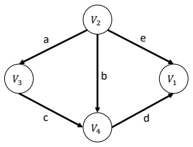
- [Section 3, Assumption 1 and Lemma 5] Assumption 1 is a no-cancellation support condition, not the standard d-separation faithfulness used in causal discovery. The proofs of Lemma 1, Lemma 5, and Theorem 15 all identify the support of a column of B' with the observed descendant set of the corresponding variable. This equivalence fails under exact cancellation of total effects. For example, in the DAG V1 -> V3 -> V2 and V1 -> V2 with structural equations V1 = N1, V3 = a V1 + N3, and V2 = b V1 + c V3 + N2, choosing b = -ac gives [B]_{2,1} = 0 even though V1 reaches V2. The n0*/n*0 test in Lemma 5 then reports no causal path from V1 to V2. If the paper intends to claim identifiability under ordinary faithfulness, this claim is unsupported; if the stronger condition is intended, it should be stated as a separate assumption (e.g., 'no-cancellation faithfulness') and its restrictiveness should be discussed explicitly.
- [Section 4.2, Theorem 15] The enumeration formula in Theorem 15 is not correct as stated because the product is computed from B'', the reduced matrix obtained after deleting columns that are proportional to other columns. Models with absorbable latent variables generate exactly the same observed distribution but are not counted. A concrete case is the model of Example 4: V3 latent, V3 -> V1 -> V2. The column of B' corresponding to N3 is proportional to the column corresponding to N1, so after absorption B'' has only the two observed columns and the product in Theorem 15 equals 1. Yet both the original latent-variable model and the equivalent two-variable model are compatible with the same Vo. More generally, latent variables with no observed descendants can be added arbitrarily without changing the observed distribution, so the set of 'all possible D's' is infinite unless the statement is restricted to minimal representations or to a fixed number of variables. The theorem needs an explicit minimality or fixed-dimension restriction, or a revised statement of what is being counted.
- [Section 4.2, proof of Theorem 15] The proof of Theorem 15 shows that each of the Pi r_i column selections can be realized by some assignment of the matrices A_oo, A_ol, A_lo, A_ll, but it does not prove completeness, i.e., it does not show that every D generating the same observed distribution corresponds to one of the enumerated selections. In particular, representations for which the associated B' is reducible are not covered by the identifiability argument based on Proposition 3. The completeness step needs to be made explicit, and in light of the previous comment it will require additional assumptions to be true.
minor comments (4)
- [Lemma 5 proof] In the proof of Lemma 5, the phrase 'there is no causal path between Vi and Vi' should read 'there is no causal path between Vi and Vj'.
- [Section 4.1] In the non-identifiability example, the sentence 'The direct causal effects from Vk to Vi, from Vk to Vj, and from Vi to Vi are α, γ, and β, respectively' should say 'from Vi to Vj' rather than 'from Vi to Vi'.
- [Section 3, paragraph before Example 4] The statement that B' is not reducible if and only if the columns of [I | Aol(I-All)^{-1}] are 'not linearly independent' is confusing and, when there are more columns than rows, trivially true. The intended condition is that no two columns are linearly dependent (pairwise linear independence), which is the definition of reducibility used in the paper.
- [Section 5] The experiments use RICA, a heuristic overcomplete ICA method, and the paper does not discuss the conditions under which RICA recovers the true mixing matrix. The empirical results should therefore be presented as illustrative rather than as a validation of the identifiability theorems.
Circularity Check
No significant circularity: the main identifiability results are derived from explicit assumptions and an external ICA theorem, with no fitted input renamed as prediction.
full rationale
The paper's derivation chain is self-contained relative to its stated assumptions. Assumption 1, which says the total causal effect is nonzero whenever a directed path exists, is an explicit hypothesis rather than a conclusion smuggled in; Lemmas 1 and 5 use it to translate support patterns of the recovered mixing matrix into ancestor/descendant relations. This is a conditional identifiability argument, not a definitional equivalence. The column-recovery step rests on an external overcomplete ICA identifiability theorem from Eriksson and Koivunen (2004), which does not depend on the present paper's fitted values. Theorem 15 counts possible total-effect matrices by choosing columns with identical descendant sets; the count follows from the stated support identification and is not a fitted parameter later called a prediction. Theorem 16's unique-identification condition is an explicit structural assumption, Assumption 2, and the non-identifiability example is credited to Hoyer et al. (2008). Self-citations appear mainly in the introduction and as background, and they are not load-bearing for the central claims. The strong no-cancellation content of Assumption 1 is a substantive limitation: if two paths cancel, Lemma 5 and Theorem 15 would fail. But the paper states that assumption explicitly rather than deriving its conclusions from its own output, so this is a correctness or applicability concern, not circularity.
Assumptions & free parameters
assumptions (4)
- domain assumption Faithfulness (Assumption 1): total causal effect [B]_{j,i} is nonzero whenever Vi to Vj is a directed path, ruling out exact cancellation of effects along multiple paths.
- domain assumption All exogenous noises are non-Gaussian.
- standard math Eriksson-Koivunen overcomplete ICA identifiability (Proposition 3): a non-reducible mixing matrix is identifiable up to column scaling and permutation.
- domain assumption The causal graph is acyclic and the structural equations are linear.
Cite this review
Pith. "Pith review of Learning Linear Non-Gaussian Causal Models in the Presence of Latent Variables." pith.science (2026). https://pith.science/paper/63GWR5V2
@misc{pith2026190803932,
  author       = {Pith},
  title        = {Pith review of: Learning Linear Non-Gaussian Causal Models in the Presence of Latent Variables},
  year         = {2026},
  howpublished = {\url{https://pith.science/paper/63GWR5V2}},
  note         = {Machine review of arXiv:1908.03932}
}
read the original abstract
We consider the problem of learning causal models from observational data generated by linear non-Gaussian acyclic causal models with latent variables. Without considering the effect of latent variables, one usually infers wrong causal relationships among the observed variables. Under faithfulness assumption, we propose a method to check whether there exists a causal path between any two observed variables. From this information, we can obtain the causal order among them. The next question is then whether or not the causal effects can be uniquely identified as well. It can be shown that causal effects among observed variables cannot be identified uniquely even under the assumptions of faithfulness and non-Gaussianity of exogenous noises. However, we will propose an efficient method to identify the set of all possible causal effects that are compatible with the observational data. Furthermore, we present some structural conditions on the causal graph under which we can learn causal effects among observed variables uniquely. We also provide necessary and sufficient graphical conditions for unique identification of the number of variables in the system. Experiments on synthetic data and real-world data show the effectiveness of our proposed algorithm on learning causal models.
Figures


Figures from the paper (4 more)


Reference graph
Works this paper leans on
-
[1]
Causality in linear nongaussian acyclic models in the presence of latent gaussian confounders
Zhitang Chen and Laiwan Chan. Causality in linear nongaussian acyclic models in the presence of latent gaussian confounders. Neural Computation, 25 0 (6): 0 1605--1641, 2013
work page 2013
-
[2]
An introduction to the bootstrap
Bradley Efron and Robert J Tibshirani. An introduction to the bootstrap. CRC press, 1994
work page 1994
-
[3]
Discovering unconfounded causal relationships using linear non-gaussian models
Doris Entner and Patrik O Hoyer. Discovering unconfounded causal relationships using linear non-gaussian models. In JSAI International Symposium on Artificial Intelligence, pages 181--195. Springer, 2010
work page 2010
-
[4]
Identifiability, separability, and uniqueness of linear ica models
Jan Eriksson and Visa Koivunen. Identifiability, separability, and uniqueness of linear ica models. IEEE signal processing letters, 11 0 (7): 0 601--604, 2004
work page 2004
-
[5]
Learning minimal latent directed information polytrees
Jalal Etesami, Negar Kiyavash, and Todd Coleman. Learning minimal latent directed information polytrees. Neural computation, 28 0 (9): 0 1723--1768, 2016
work page 2016
-
[6]
Budgeted experiment design for causal structure learning
AmirEmad Ghassami, Saber Salehkaleybar, Negar Kiyavash, and Elias Bareinboim. Budgeted experiment design for causal structure learning. In International Conference on Machine Learning, pages 1724--1733, 2018
work page 2018
-
[7]
Estimation of causal effects using linear non-gaussian causal models with hidden variables
Patrik O Hoyer, Shohei Shimizu, Antti J Kerminen, and Markus Palviainen. Estimation of causal effects using linear non-gaussian causal models with hidden variables. International Journal of Approximate Reasoning, 49 0 (2): 0 362--378, 2008
work page 2008
-
[8]
Nonlinear causal discovery with additive noise models
Patrik O Hoyer, Dominik Janzing, Joris M Mooij, Jonas Peters, and Bernhard Sch \"o lkopf. Nonlinear causal discovery with additive noise models. In Advances in neural information processing systems, pages 689--696, 2009
work page 2009
Show all 24 references
-
[9]
Independent component analysis, volume 46
Aapo Hyv \"a rinen, Juha Karhunen, and Erkki Oja. Independent component analysis, volume 46. John Wiley & Sons, 2004
2004
-
[10]
Estimation of a structural vector autoregression model using non-gaussianity
Aapo Hyv \"a rinen, Kun Zhang, Shohei Shimizu, and Patrik O Hoyer. Estimation of a structural vector autoregression model using non-gaussianity. Journal of Machine Learning Research, 11 0 (May): 0 1709--1731, 2010
2010
-
[11]
Information-geometric approach to inferring causal directions
Dominik Janzing, Joris Mooij, Kun Zhang, Jan Lemeire, Jakob Zscheischler, Povilas Daniu s is, Bastian Steudel, and Bernhard Sch \"o lkopf. Information-geometric approach to inferring causal directions. Artificial Intelligence, 182: 0 1--31, 2012
2012
-
[12]
Ica with reconstruction cost for efficient overcomplete feature learning
Quoc V Le, Alexandre Karpenko, Jiquan Ngiam, and Andrew Y Ng. Ica with reconstruction cost for efficient overcomplete feature learning. In Advances in neural information processing systems, pages 1017--1025, 2011
2011
-
[13]
Probabilistic Reasoning in Intelligent Systems: Networks of Plausible Inference
Judea Pearl. Probabilistic Reasoning in Intelligent Systems: Networks of Plausible Inference. Morgan Kaufmann, 1988
1988
-
[14]
Causality
Judea Pearl. Causality. Cambridge university press, 2009
2009
-
[15]
Identifiability of gaussian structural equation models with equal error variances
Jonas Peters and Peter B \"u hlmann. Identifiability of gaussian structural equation models with equal error variances. Biometrika, 101 0 (1): 0 219--228, 2013
2013
-
[16]
Causal inference by using invariant prediction: identification and confidence intervals
Jonas Peters, Peter B \"u hlmann, and Nicolai Meinshausen. Causal inference by using invariant prediction: identification and confidence intervals. Journal of the Royal Statistical Society: Series B (Statistical Methodology), 78 0 (5): 0 947--1012, 2016
2016
-
[17]
Learning vector autoregressive models with latent processes
Saber Salehkaleybar, Jalal Etesami, Negar Kiyavash, and Kun Zhang. Learning vector autoregressive models with latent processes. In International Conference on Machine Learning, pages 4000--4007, 2018
2018
-
[18]
Bayesian estimation of causal direction in acyclic structural equation models with individual-specific confounder variables and non-gaussian distributions
Shohei Shimizu and Kenneth Bollen. Bayesian estimation of causal direction in acyclic structural equation models with individual-specific confounder variables and non-gaussian distributions. The Journal of Machine Learning Research, 15 0 (1): 0 2629--2652, 2014
2014
-
[19]
A linear non-gaussian acyclic model for causal discovery
Shohei Shimizu, Patrik O Hoyer, Aapo Hyv \"a rinen, and Antti Kerminen. A linear non-gaussian acyclic model for causal discovery. Journal of Machine Learning Research, 7 0 (Oct): 0 2003--2030, 2006
2003
-
[20]
Directlingam: A direct method for learning a linear non-gaussian structural equation model
Shohei Shimizu, Takanori Inazumi, Yasuhiro Sogawa, Aapo Hyv \"a rinen, Yoshinobu Kawahara, Takashi Washio, Patrik O Hoyer, and Kenneth Bollen. Directlingam: A direct method for learning a linear non-gaussian structural equation model. Journal of Machine Learning Research, 12 0...
2011
-
[21]
Causation, prediction, and search
Peter Spirtes, Clark N Glymour, Richard Scheines, David Heckerman, Christopher Meek, Gregory Cooper, and Thomas Richardson. Causation, prediction, and search. MIT press, 2000
2000
-
[22]
Parcelingam: a causal ordering method robust against latent confounders
Tatsuya Tashiro, Shohei Shimizu, Aapo Hyv \"a rinen, and Takashi Washio. Parcelingam: a causal ordering method robust against latent confounders. Neural computation, 26 0 (1): 0 57--83, 2014
2014
-
[23]
On the identifiability of the post-nonlinear causal model
Kun Zhang and Aapo Hyv \"a rinen. On the identifiability of the post-nonlinear causal model. In Proceedings of the twenty-fifth conference on uncertainty in artificial intelligence, pages 647--655. AUAI Press, 2009
2009
-
[24]
Causal discovery in the presence of distribution shift: Skeleton estimation and orientation determination
Kun Zhang, Biwei Huang, Jiji Zhang, Clark Glymour, and Bernhard Sch \"o lkopf. Causal discovery in the presence of distribution shift: Skeleton estimation and orientation determination. In Proc. International Joint Conference on Artificial Intelligence (IJCAI 2017), 2017
2017
Reviewed August 14, 2026 · model on record in the stance chip above.
Discussion (0). Continue with ORCID to comment.