REVIEW 4 major objections 5 minor 66 references
WWhittle Maximum Likelihood Estimate of spectral properties of Rayleigh-Taylor interfacial mixing using hot-wire anemometry experimental data
T0 review · 4 major / 5 minor · reviewed 2026-08-14 · deepseek-v4-flash
Pith's one-line read The velocity-fluctuation spectrum in pure Rayleigh-Taylor mixing fits a power law times an exponential.
desk verdict The statistics are careful and the cutoff-dependence maps are useful, but the central comparison with group theory depends on an unstated Taylor-hypothesis mapping that the paper never justifies. read the letter →
The pith
A machine-rendered reading of the paper's core claim, the machinery that carries it, and where it could break.
The reading
What carries the argument
The machinery is Whittle's maximum likelihood estimator for periodogram fitting. It treats each periodogram ordinate $2I_k/S(k)$ as an approximately independent chi-square random variable with two degrees of freedom, builds the quasi-log-likelihood $\ln L = -\sum_k [\ln S(k)+I_k/S(k)]$, and maximizes it over the parameters $(\alpha,\beta,\gamma)$ of the model $S(k)=C k^{\alpha} e^{\beta k}+S_{\mathrm{noise}}$ via Newton-Raphson iteration. The Hessian of the log-likelihood supplies the Fisher information matrix, from which the parameter error bars are computed, and the Kolmogorov-Smirnov test on the residuals $Y_k=2I_k/S(k)$ provides the goodness-of-fit criterion. This machinery converts a raw time series into parameter estimates, error bars and a statistical rejection test in one pipeline.
What would settle it
Split the 50-second record into two halves, compute the periodogram and the Whittle MLE separately on each half, and compare the fitted $\alpha$ and $\beta$: if the two halves give parameters that differ by more than the quoted error bars, the stationarity assumption fails and the fitted spectrum is not a well-defined property of the flow.
Extended reading notes
Core claim
The central discovery is that the measured velocity-fluctuation spectrum in late-time pure Rayleigh-Taylor mixing is not a pure power law but the product of a power law and an exponential decay, $S(k)=C k^{\alpha} \exp(\beta k)$, with a flat instrumental-noise floor at high wavevectors. For the $v$ component of velocity the maximum-likelihood estimate gives $\alpha=-2.04$ with a relative error of about 3.6 percent and $\beta=-1\times 10^{-3}$ with a relative error of about 6.4 percent over the fitting range $k=101$ to $3000$. The paper interprets the closeness of $\alpha$ to $-2$ as agreement with the group-theory spectrum for Rayleigh-Taylor mixing, and the exponential length scale $|\beta|^{-1}\approx 1000$ as comparable to the viscous scale $k_\nu$, indicating a physical rather than instrumental origin. It also reports that the fit is robust over a domain of left and right cutoffs where relative errors are below 10 percent and the Kolmogorov-Smirnov p-value exceeds 50 percent, and that applying moving-average smoothing to the periodogram leaves the parameter estimates unchanged but makes the KS test reject the fit, so raw data must be used.
Load-bearing premise
The load-bearing premise is that the 50-second hot-wire record is a zero-mean stationary time series whose periodogram ordinates are independent and chi-square distributed, even though Rayleigh-Taylor mixing is anisotropic, inhomogeneous and statistically unsteady.
Editorial extensions
If this is right
- If the compound spectrum is right, the Rayleigh-Taylor spectrum is steeper than the $-5/3$ law of canonical turbulence and consistent with the $-2$ law from group theory in the self-similar range.
- The exponential term sets a finite characteristic scale comparable to the viscous scale, so the pure power law is only an intermediate-range description.
- Accurate determination of the power-law exponent requires including enough high-wavevector modes, while accurate determination of the exponential decay requires enough low-wavevector modes.
- Smoothing a periodogram before fitting does not change the estimated parameters but destroys the statistical validity of the fit, so raw unprocessed data are preferable.
- The same estimator can be applied to other velocity components and to density fluctuations, where the fitted parameters should differ and thereby quantify anisotropy and sensitivity to deterministic conditions.
Reading between the lines
- If the compound form is generic, longer records or cleaner experiments should show $\alpha$ converging toward $-2$ and $|\beta|$ shrinking as the dynamic range widens; a testable prediction is that $k^{-\alpha} S(k)$ should approach a pure exponential with a constant scale.
- The KS failure on smoothed spectra suggests that visual inspection of smoothed RT spectra can manufacture apparent agreement with scaling laws; quantitative residual tests should accompany every reported spectral exponent.
- The same pipeline could be run on simulation data for RT mixing or on Kelvin-Helmholtz and convection experiments; if the compound form persists with different $(\alpha,\beta)$, it would give a statistical fingerprint distinguishing mixing regimes.
- Replacing the ad hoc white-noise floor with a measured instrument-noise spectrum could test whether the quoted $\alpha$ and $\beta$ are biased; if they shift outside the quoted errors, the noise model is the limiting assumption.
Signed reviews
Editorial analysis
A structured set of objections, weighed in public.
Referee Report
Summary. The paper proposes a Whittle-maximum-likelihood method to estimate the parameters of a compound spectral model, S(k)=C k^alpha exp(beta k) plus a white-noise floor, from a 50 s hot-wire time series of the v velocity component in the 'pure' Rayleigh-Taylor setup A1S0 of Akula et al. (2017). The authors compute the periodogram from N=5e4 samples, derive the gradient and Hessian of the quasi-log-likelihood, obtain the maximum-likelihood estimates by Newton-Raphson, estimate parameter errors from the Hessian, and use a Kolmogorov-Smirnov test on the periodogram-to-model ratios to assess goodness-of-fit. For the fitting window k=101-3000 with S_noise=1e-7, they report alpha=-2.04 with a 3.6% relative error, beta=-1e-3 with a 6.4% relative error, and pKS=43.6%, and they interpret these results as consistency with the group-theory spatial spectrum S(k)~k^-2 and with a viscous cutoff near k_nu. They also study how alpha, beta, their errors, and the KS p-value vary with the left and right cutoffs, and they compare the compound fit with a pure power-law fit.
Significance. If the central claim is established, the paper makes a useful methodological contribution: it applies a rigorous statistical estimation procedure to raw experimental RT data, includes a goodness-of-fit test that correctly rejects smoothed periodograms, and provides a systematic study of the dependence of fitted parameters on the fitting window. The derivation of the likelihood, gradient, and Hessian is clear and internally consistent, and the use of raw rather than smoothed data is a sensible and well-demonstrated choice. The main value of the paper is therefore in the method and in the cautionary demonstration that visual inspection of smoothed spectra can be misleading. However, the physical conclusion that the fitted exponent and decay rate confirm group-theory predictions is currently not supported by the manuscript because of missing frequency-to-wavenumber mapping, an apparently incorrect 1/N factor in the error estimates, and the post-fit nature of the comparison with theory.
major comments (4)
- [§III.2, Eq. (3); §IV.3] The index k in Eq. (3) is introduced as the DFT index in Eq. (1), i.e., as a temporal frequency index f=k/(N dt), but the central claim compares the fitted exponent with the spatial spectrum S(k)~k^-2 and compares 1/beta with the viscous wavenumber k_nu. No Taylor/frozen-flow mapping k_phys=2*pi*f/U and no mean convection velocity U are stated or justified. Without this mapping, the fitted alpha is a temporal-spectrum exponent, and the dimensional comparison in §IV.3 (k*=(beta* H)^-1=8.33e2 m^-1 versus k_nu~1.1e3 m^-1) is not grounded. The authors should either state and verify the conversion (including the value of U) or explicitly reframe the result as a temporal-spectrum analysis.
- [§III.3, after Eq. (7)] The covariance formula Cov(bold theta)≈-H^{-1}(bold theta)/N and sigma_i=sqrt(-H^{-1}_{ii}/N) divides the inverse observed Hessian by the total sample size N=5e4. The Hessian in Eq. (6) is already a sum over the eta=kr-kl+1 fitted periodogram ordinates, not over N time samples; the asymptotic covariance of the Whittle MLE is approximately (-E[H])^{-1} without an additional 1/N factor. The reported relative errors (3.6% for alpha and 6.4% for beta) are therefore understated by a factor of order sqrt(N), and the 'relative error less than 10%' criterion used to select the confidence domain in Figs. 6-9 is not reliable.
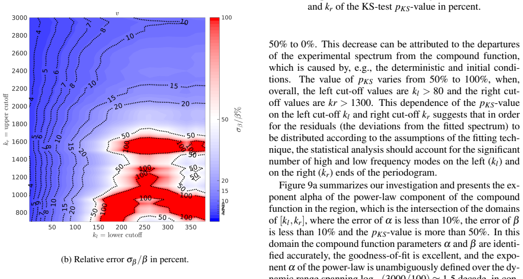
- [§IV.2, §IV.3, Fig. 9] The KS test is applied to the fitted model and therefore tests whether the periodogram ordinates are consistent with the assumed compound spectrum; it does not test whether the group-theory values alpha=-2 and beta=-1/k_nu are correct. The agreement claimed in §IV.3 is a post-fit comparison: alpha and beta are estimated from the same periodogram that is then compared with theory. Moreover, the quoted 6.4% error on beta corresponds to k* values in the range [783,891] m^-1, whereas k_nu is in [1080,1130] m^-1, so the ratio k_nu/k*=1.29-1.35 is outside the stated uncertainty. The authors should report confidence intervals for alpha and beta and test the hypotheses alpha=-2 and beta=-1/k_nu directly, or via a likelihood-ratio comparison with the unconstrained compound model.
- [§III.2; §VI (Discussion)] The estimator is derived under the assumption that X_j is a zero-mean stationary time series whose periodogram ordinates are asymptotically independent and chi-squared distributed, yet the paper nowhere tests stationarity or the absence of trends in the 50 s record. The Discussion itself concedes that maximum-likelihood requirements 'may be challenging to obey' in Rayleigh-Taylor mixing. Because the KS p-value and the error bars both rely on this assumption, the paper should include at least a basic stationarity check (e.g., split-sample fits, trend removal, or a test for time-varying variance) before pKS=43.6% can be interpreted as evidence for the model.
minor comments (5)
- [§IV.1] The text contains several typographical errors, including 'desribing', 'deterministric', 'viscuous', and 'demonstrably distrinct'; these should be corrected throughout.
- [§III.3] The phrase 'the tolerable accuracy being less that ~10% for relative errors in physics experiments' is vague and should be replaced by a quantitative, justified criterion.
- [§IV.1] The noise floor S_noise=1e-7 is selected as 'visually consistent with the data' and no sensitivity analysis with respect to S_noise is reported; a short scan over S_noise would strengthen the claim that the fitted alpha and beta are robust to this choice.
- [§IV.3, Fig. 9] The criteria used to define the 'confidence domain' (errors below 10% and pKS above 50% in Fig. 9a; errors below 20% and pKS above 5% in Fig. 9b) are arbitrary; the authors should justify these thresholds or present the underlying distributions of alpha and beta.
- [§II.3, §IV.3] The claim that k* is 'in agreement with the theory' would be better phrased as 'comparable to k_nu within the limitations of the model', given the discrepancy of about 30% between k* and k_nu.
Circularity Check
No significant circularity: alpha and beta are free MLE parameters; the group-theory comparison is an out-of-sample consistency check, not a construction.
full rationale
The paper's derivation chain is a standard statistical fit. Equation (3) defines the model S_RT(k)=C k^alpha exp(beta k), with alpha, beta, and gamma as free parameters estimated by maximizing the Whittle quasi-log-likelihood (Eqs. 5-7). The Newton-Raphson iteration and Fisher-information errors do not import the group-theory values -2 or k_nu; the theory enters only through the choice of model form and through the final comparisons. In particular, the claimed alpha=-2.04 and beta=-1e-3 are outputs of the fit, and the KS p-value of 43.6% is a nontrivial goodness-of-fit result for the raw-data residuals against chi-square_2. The comparison k*=(beta* H)^-1 ~ k_nu is a post-fit consistency check using the fitted beta, not a parameter set to that value; it could have failed. The use of the compound ansatz is motivated by prior group-theory work, some of which is self-cited (e.g., [3,4,23,24]), but that motivation does not make the fitted exponents equal to the theory by construction. The Discussion explicitly lists the limitations of stationarity and Whittle-approximation requirements for RT mixing; these are statistical assumptions whose violation would affect validity, but they do not render the derivation circular. The unstated conversion from DFT frequency index to physical wavenumber is a mapping/correctness concern, not a circular reduction: no equation in the paper forces k in Eq. (3) to equal k_phys H, and the fitted alpha would remain a fit even if the mapping were wrong. Therefore no step reduces to its own input; score 0.
Assumptions & free parameters
free parameters (5)
- alpha (power-law exponent) =
-2.04 (MLE fit, v component, k=101-3000)
- beta (exponential decay rate) =
-1.0e-3 (MLE fit; later quoted as beta*=1.00e-3)
- gamma (log amplitude C) =
not reported
- SNoise (white noise floor) =
1e-7
- fitting window cutoffs kl, kr =
kl=101, kr=3000 for headline fit; scanned broadly
assumptions (5)
- standard math Fourier coefficients of a zero-mean stationary time series are asymptotically independent and Gaussian with variance S(k), so Y_k=2I_k/S(k) follows chi-square_2.
- domain assumption The 50 second experimental record is a zero-mean stationary near-Gaussian signal.
- ad hoc to paper The RT spectral component has the compound form SRT(k)=C k^alpha e^{beta k}.
- domain assumption The instrumental noise is white and constant at level SNoise ~ 1e-7.
- domain assumption The v-component of velocity is the least affected by deterministic experimental conditions.
Cite this review
Pith. "Pith review of WWhittle Maximum Likelihood Estimate of spectral properties of Rayleigh-Taylor interfacial mixing using hot-wire anemometry experimental data." pith.science (2026). https://pith.science/paper/KZ2MC243
@misc{pith2026190803977,
  author       = {Pith},
  title        = {Pith review of: WWhittle Maximum Likelihood Estimate of spectral properties of Rayleigh-Taylor interfacial mixing using hot-wire anemometry experimental data},
  year         = {2026},
  howpublished = {\url{https://pith.science/paper/KZ2MC243}},
  note         = {Machine review of arXiv:1908.03977}
}
read the original abstract
Investigating the power density spectrum of fluctuations in Rayleigh-Taylor (RT) interfacial mixing is a means of studying characteristic length- and time-scales, anisotropies and anomalous processes. Guided by group theory, analysing the invariance-based properties of the fluctuations, our work examines raw time series from hot-wire anemometry measurements in the experiment by Akula et al., JFM 816, 619-660 (2017). The results suggest that the power density spectrum can be modelled as a compound function presented as the product of a power law and an exponential. The data analysis is based on Whittle's approximation of the power density spectrum for independent zero-mean near-Gaussian signals to construct a Maximum likelihood Estimator (MLE) of the parameters. Those that maximise the log-likelihood are computed numerically through Newton-Raphson iteration. The Hessian of the log-likelihood is used to evaluate the Fisher information matrix and provide an estimate of the statistical error on the obtained parameters. The Kolmogorov-Smirnov test is applied to analyse the goodness-of-fit, by verifying the hypothesis that the ratio between the observed periodogram and the estimated power density spectrum follows a chi-squared probability distribution. The dependence of the parameters of the compound function is investigated on the range of mode numbers over which the fit is performed. In the domain where the relative errors of the power law exponent and the exponential decay rate are small and the goodness-of-fit is excellent, the parameters of the compound function are clearly defined, in agreement with the theory. The study of the power-law spectra in RT mixing data suggests that rigorous physics-based statistical methods can help researchers to see beyond visual inspection.
Figures



Figures from the paper (9 more)




Reference graph
Works this paper leans on
-
[1]
J. W. Strutt (3rd Baron Rayleigh), Proceedings of the London Mathematical Society s1-14, 170 (1883)
-
[2]
The α and β estimates being positions of maximum like- lihood, their variation is correlated with respect to changes in parameters such as kl and kr. The correlation can be under- stood by considering the log of the power density spectrum lnSRT = α lnk + βk + γ as the weighted sum of the three basic functions ln k, k and 1, where the power-law has an influ...
work page 2000
-
[3]
S. I. Abarzhi, Philosophical Transactions of the Royal Society A: Mathematical, Physical and Engineering Sciences 368, 1809 (2010)
work page 2010
-
[4]
R. M. Davies and G. I. Taylor, Proceedings of the Royal Society of London. Series A. Mathematical and Physical Sciences 200, 375 (1950)
work page 1950
-
[5]
E. E. Meshkov, Studies of hydrodynamic instabilities in labora- tory experiments (Sarov, FGUC-VNIIEF, ISBN 5-9515-0069-9, in Russian, 2006)
work page 2006
-
[6]
([2017]). In the experiments [6], the fluids with different densities first co-flow in separate channels parallel to one another, in fluid streams with the same or with different speeds, and with the heavy fluid positioned above the light fluid. Next, at the end of the channels, the fluid streams meet, the unstable in- terface between the fluids forms, the initia...
work page 2017
-
[7]
S. I. Abarzhi, EPL (Europhysics Letters) 91, 35001 (2010)
work page 2010
- [8]
Show all 66 references
-
[9]
Akula and D
B. Akula and D. Ranjan, Journal of Fluid Mechanics 795, 313–355 (2016)
2016
-
[10]
S. I. Abarzhi, S. Gauthier, and K. R. Sreenivasan, Philosophical Transactions of the Royal Society A: Mathematical, Physical and Engineering Sciences 371, 20120436 (2013)
2013
-
[11]
W. D. Arnett, Supernovae and Nucleosynthesis: An Investiga- tion of the History of Matter, from the Big Bang to the Present, Princeton Series in Astrophysics (Princeton University Press, 1996)
1996
-
[12]
S. W. Haan, J. D. Lindl, D. A. Callahan, D. S. Clark, J. D. Salmonson, B. A. Hammel, L. J. Atherton, R. C. Cook, M. J. Edwards, S. Glenzer, A. V . Hamza, S. P. Hatchett, M. C. Her- rmann, D. E. Hinkel, D. D. Ho, H. Huang, O. S. Jones, J. Kline, G. Kyrala, O. L. Landen, B. J. M...
2011
-
[13]
Peters, Turbulent Combustion, Cambridge Monographs on Mechanics (Cambridge University Press, 2000)
N. Peters, Turbulent Combustion, Cambridge Monographs on Mechanics (Cambridge University Press, 2000)
2000
-
[14]
S. I. Anisimov, R. P. Drake, S. Gauthier, E. E. Meshkov, and S. I. Abarzhi, Philosophical Transactions of the Royal Soci- ety A: Mathematical, Physical and Engineering Sciences 371, 20130266 (2013)
2013
-
[15]
S. S. Orlov, S. I. Abarzhi, S. B. Oh, G. Barbastathis, and K. R. Sreenivasan, Philosophical Transactions of the Royal Society A: Mathematical, Physical and Engineering Sciences 368, 1705 (2010)
2010
-
[16]
K. R. Sreenivasan, Proceedings of the National Academy of Sci- ences of the USA (2018), 10.1073/pnas.1800463115
2018 doi
-
[17]
E. E. Meshkov, Philosophical Transactions of the Royal Soci- ety A: Mathematical, Physical and Engineering Sciences 371, 20120288 (2013)
2013
-
[18]
H. F. Robey, Y . Zhou, A. C. Buckingham, P. Keiter, B. A. Rem- ington, and R. P. Drake, Physics of Plasmas 10, 614 (2003)
2003
-
[19]
B. A. Remington, H.-S. Park, D. T. Casey, R. M. Cavallo, D. S. Clark, C. M. Huntington, C. C. Kuranz, A. R. Miles, S. R. Nagel, K. S. Raman, and V . A. Smalyuk, Proceedings of the National Academy of Sciences of the USA (2018), 10.1073/pnas.1717236115
2018 doi
-
[20]
J. R. Ristorcelli and T. T. Clark, Journal of Fluid Mechanics507, 213–253 (2004)
2004
-
[21]
Glimm, D
J. Glimm, D. H. Sharp, T. Kaman, and H. Lim, Philosophical Transactions of the Royal Society A: Mathematical, Physical and Engineering Sciences 371, 20120183 (2013)
2013
-
[22]
Kadau, J
K. Kadau, J. L. Barber, T. C. Germann, B. L. Holian, and B. J. Alder, Philosophical Transactions of the Royal Society A: Mathematical, Physical and Engineering Sciences 368, 1547 (2010)
2010
-
[23]
D. L. Youngs, Philosophical Transactions of the Royal Soci- ety A: Mathematical, Physical and Engineering Sciences 371, 20120173 (2013)
2013
-
[24]
S. I. Abarzhi, A. Gorobets, and K. R. Sreenivasan, Physics of Fluids 17, 081705 (2005)
2005
-
[25]
E. E. Meshkov and S. I. Abarzhi, Fluid Dynamics Research 51, 065502 (2019)
2019
-
[26]
S. I. Abarzhi, A. K. Bhowmick, A. Naveh, A. Pandian, N. C. Swisher, R. F. Stellingwerf, and W. D. Arnett, Proceedings of the National Academy of Sciences 116, 18184 (2019)
2019
-
[27]
A. N. Kolmogorov, Giornale dell’Istituto Italiano degli Attuari 4, 83 (1933)
1933
-
[28]
Smirnov, Ann
N. Smirnov, Ann. Math. Statist. 19, 279 (1948)
1948
-
[29]
Kolmogorov, Dokl
A. Kolmogorov, Dokl. Akad. Nauk SSSR 30, 299 (1941)
1941
-
[30]
Kolmogorov, Dokl
A. Kolmogorov, Dokl. Akad. Nauk SSSR 31, 538 (1941)
1941
-
[31]
Landau and E
L. Landau and E. Lifshitz, Course of theoretical physics , V ol. I-X (Elsevier Science, 1987)
1987
-
[32]
K. R. Sreenivasan, Rev. Mod. Phys. 71, S383 (1999)
1999
-
[33]
Ruddick, A
B. Ruddick, A. Anis, and K. Thompson, Journal of Atmo- spheric and Oceanic Technology 17, 1541 (2000)
2000
-
[34]
Vaughan, S., A&A 431, 391 (2005)
2005
-
[35]
C. E. Bluteau, N. L. Jones, and G. N. Ivey, Limnology and Oceanography: Methods 9, 302 (2011). 13
2011
-
[36]
Choudhuri, S
N. Choudhuri, S. Ghosal, and A. Roy, Journal of the American Statistical Association 99, 1050 (2004)
2004
-
[37]
R. H. Kraichnan, Journal of Fluid Mechanics 5, 497–543 (1959)
1959
-
[38]
K. R. Sreenivasan, The Physics of Fluids 27, 1048 (1984)
1984
-
[39]
S. G. Saddoughi and S. V . Veeravalli, Journal of Fluid Mechan- ics 268, 333–372 (1994)
1994
-
[40]
Khurshid, D
S. Khurshid, D. A. Donzis, and K. R. Sreenivasan, Phys. Rev. Fluids 3, 082601 (2018)
2018
-
[41]
Distributed chaos and turbulence in bénard-marangoni and rayleigh-bénard convection,
A. Bershadskii, “Distributed chaos and turbulence in bénard-marangoni and rayleigh-bénard convection,” (2019), arXiv:1903.05018 [physics.flu-dyn]
2019 arXiv
-
[42]
Contreras-Cristán, E
A. Contreras-Cristán, E. Gutiérrez-Peña, and S. G. Walker, Communications in Statistics - Simulation and Computation35, 857 (2006)
2006
-
[43]
Brillinger, Time Series: Data Analysis and Theory , Clas- sics in Applied Mathematics (Society for Industrial and Applied Mathematics, 2001)
D. Brillinger, Time Series: Data Analysis and Theory , Clas- sics in Applied Mathematics (Society for Industrial and Applied Mathematics, 2001)
2001
-
[44]
Whittle, Journal of the Royal Statistical Society19, 38 (1957)
P. Whittle, Journal of the Royal Statistical Society19, 38 (1957)
1957
-
[45]
F. J. Massey, Journal of the American Statistical Association46, 68 (1951)
1951
-
[46]
K. O. Mikaelian, Physica D: Nonlinear Phenomena 36, 343 (1989)
1989
-
[47]
Zhou, Physics of Fluids13, 538 (2001)
Y . Zhou, Physics of Fluids13, 538 (2001)
2001
-
[48]
A. M. Obukhov and A. M. Yaglom, Quarterly Journal of the Royal Meteorological Society 85, 81 (1959)
1959
-
[49]
Bolgiano Jr., Journal of Geophysical Research (1896-1977) 64, 2226 (1959)
R. Bolgiano Jr., Journal of Geophysical Research (1896-1977) 64, 2226 (1959)
1959
-
[50]
G. K. Batchelor, The Physics of Fluids 12, II (1969)
1969
-
[51]
Akula, Experimental Investigation of Buoyancy Driven Mix- ing With and Without Shear at Different Atwood Numbers, Ph.D
B. Akula, Experimental Investigation of Buoyancy Driven Mix- ing With and Without Shear at Different Atwood Numbers, Ph.D. thesis, Texas A & M University (2014)
2014
-
[52]
W. N. Kraft, A. Banerjee, and M. J. Andrews, Experiments in Fluids 47, 49 (2009)
2009
-
[53]
G. I. Taylor, Proceedings of the Royal Society of London 201, 175 (1950)
1950
-
[54]
D. D. Ryutov, M. S. Derzon, and M. K. Matzen, Rev. Mod. Phys. 72, 167 (2000)
2000
-
[55]
Gekelman, B
W. Gekelman, B. V . Compernolle, T. DeHaas, and S. Vincena, Plasma Physics and Controlled Fusion 56, 064002 (2014)
2014
-
[56]
Kolmogorov, Dokl
A. Kolmogorov, Dokl. Akad. Nauk SSSR 32, 19 (1941)
1941
-
[57]
A. N. Kolmogorov, Proceedings: Mathematical and Physical Sciences 434, 9 (1991)
1991
-
[58]
Bandt and B
C. Bandt and B. Pompe, Phys. Rev. Lett. 88, 174102 (2002)
2002
-
[59]
O. A. Rosso, H. A. Larrondo, M. T. Martin, A. Plastino, and M. A. Fuentes, Phys. Rev. Lett. 99, 154102 (2007)
2007
-
[60]
J. E. Maggs and G. J. Morales, Plasma Physics and Controlled Fusion 55, 085015 (2013)
2013
-
[61]
López-Ruiz, H
R. López-Ruiz, H. Mancini, and X. Calbet, Physics Letters A 209, 321 (1995)
1995
-
[62]
Martin, A
M. Martin, A. Plastino, and O. Rosso, Physica A: Statistical Mechanics and its Applications 369, 439 (2006)
2006
-
[63]
Bauke, The European Physical Journal B 58, 167 (2007)
H. Bauke, The European Physical Journal B 58, 167 (2007)
2007
-
[64]
M. J. Buehler, H. Tang, A. C. T. van Duin, and W. A. Goddard, Phys. Rev. Lett. 99, 165502 (2007)
2007
-
[65]
Rana and M
S. Rana and M. Herrmann, Physics of Fluids23, 091109 (2011)
2011
-
[66]
V . E. Neuvazhaev, Soviet Physics Doklady20, 1053 (1975). 14
1975
Reviewed August 14, 2026 · model on record in the stance chip above.
Discussion (0). Continue with ORCID to comment.