REVIEW 3 major objections 6 minor 30 references
Component-based regularisation of multivariate generalised linear mixed models
T0 review · 3 major / 6 minor · reviewed 2026-08-14 · deepseek-v4-flash
Pith's one-line read Mixed-SCGLR extends supervised-component regression to grouped-data GLMMs, recovering latent predictor bundles while regularising the fixed effects.
desk verdict A solid, honest extension of SCGLR to GLMMs, but the method is heuristic and the component criterion may confound random effects with fixed structure. read the letter →
The pith
A machine-rendered reading of the paper's core claim, the machinery that carries it, and where it could break.
The reading
What carries the argument
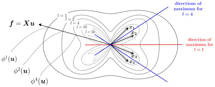
The load-bearing object is the mixed-SCGLR criterion $s\log\varphi(u) + (1-s)\log\psi_A(u)$, maximised over loading vectors $u$ under $u^T M^{-1} u = 1$ and, for higher-rank components, under orthogonality constraints. Here $\psi_A(u)$ is the goodness-of-fit of component $f = Xu$ together with the additional variables $A$ for all responses, measured by weighted cosines between each response's Schall working variable and the spanned space with the response's weight matrix; $\varphi(u)$ is the structural-relevance criterion, a weighted generalised average of squared correlations between $f$ and the original predictors, whose locality is tuned by $l$. This criterion is what makes the regularisation component-based rather than penalty-based: instead of shrinking coefficient norms, it pushes components toward interpretable bundles while preserving predictive fit. Schall's linearisation converts each conditional GLMM into a working linear mixed model, Henderson's equations update parameters and variance components, and the Projected Iterated Normed Gradient (PING) algorithm solves the constrained maximisation on the unit sphere.
What would settle it
Simulate grouped binary data from a known latent structure, fit the same data with mixed-SCGLR and with a GLMM estimated by adaptive Gauss-Hermite quadrature, and compare the first estimated component direction and the variance-component estimate across many replications; if the component direction shifts materially while the variance-component estimate is biased toward zero, Schall's linearisation is the approximation that needs replacing.
Extended reading notes
Core claim
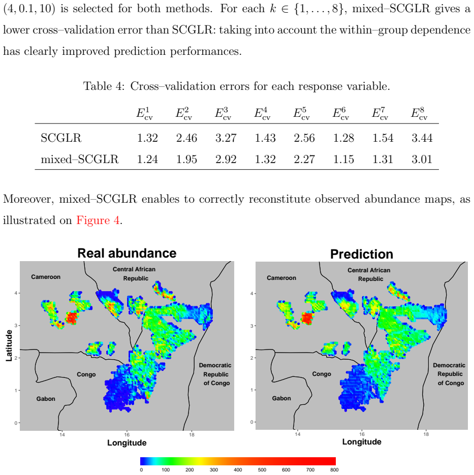
The paper establishes that the SCGLR supervised-component criterion, which trades goodness of fit against structural relevance of a component in the predictor space, can be transplanted into Schall's iterative linearisation of a GLMM. The algorithm alternates between computing a component $f = Xu$ that maximises the combined criterion on current working variables and weights, and solving Henderson mixed-model equations that update fixed effects, random-effect predictions, and variance components; the working variables and weights are then recomputed and the cycle repeats until stability. The reported simulations show that mixed-SCGLR recovers the predictive variable bundles on grouped data, even when a higher-inertia nuisance bundle is present, and that its fixed-effect estimates are the most accurate of the compared methods under strong within-bundle correlation. On the real data, mixed-SCGLR outperforms SCGLR on every response, showing that the random-effect term contributes to prediction rather than merely adjusting standard errors.
Load-bearing premise
The load-bearing premise is that Schall's linearisation, a penalised-quasi-likelihood-style approximation of the GLMM, is faithful enough that the working variables and weights still point toward the true latent explanatory dimensions; if the linearisation distorts the conditional model, the component directions, fixed-effect estimates, and variance-component updates can all be affected.
Editorial extensions
If this is right
- With strongly redundant predictors arranged in bundles, component-based regularisation of a multivariate GLMM can give lower fixed-effect estimation error than ridge or LASSO, and the advantage grows with the within-bundle correlation $\tau$.
- Modelling within-group dependence is part of the predictive gain: on grouped data, mixed-SCGLR can beat non-mixed SCGLR for every response, as in the forest census.
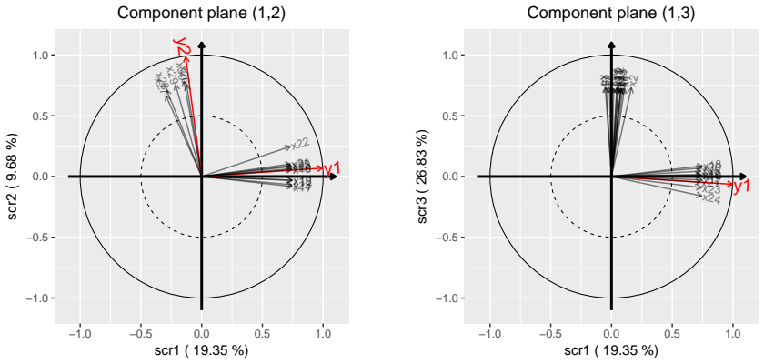
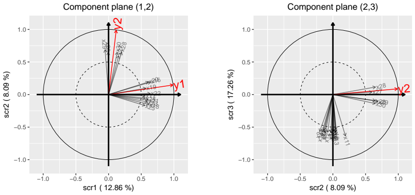
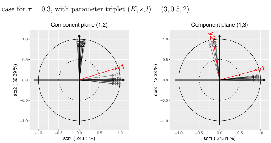
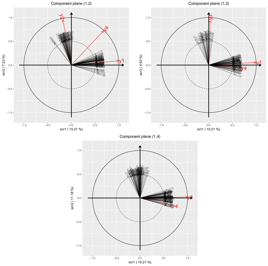
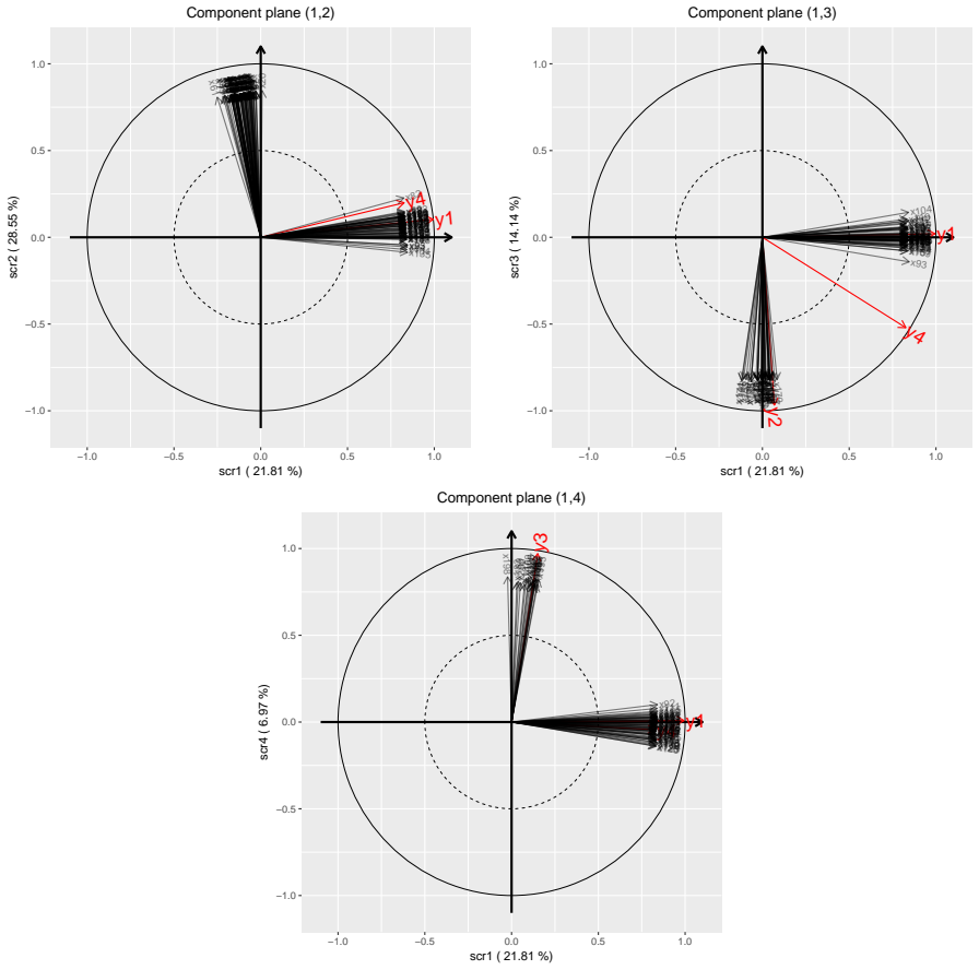
- Mixed-SCGLR yields interpretable output: component planes separate predictive bundles from high-inertia nuisance bundles, and the decomposition of each response's linear predictor onto common components reveals which responses share an explanatory dimension.
- The same algorithm handles Gaussian, Bernoulli, binomial and Poisson responses, and its high-dimensional variant (using principal components of $X$) extends the approach to $p>n$ settings.
- Because variance-component estimates from Schall's linearisation are biased toward zero for binary data, the paper anticipates that combined strategies, building components on the linearised model and estimating parameters by Monte Carlo methods, will be more reliable in that case.
Reading between the lines
- A natural next experiment is to replace only the parameter-estimation block of Algorithm 1 with a Laplace or MCMC fit while keeping the component-building step fixed; if component directions barely change, the component criterion is robust to the linearisation and the bias is concentrated in the variance components.
- When responses are driven by disjoint rather than shared predictor bundles, the common-component formulation could inflate the number of components needed; a simulation with disjoint structures would quantify that cost.
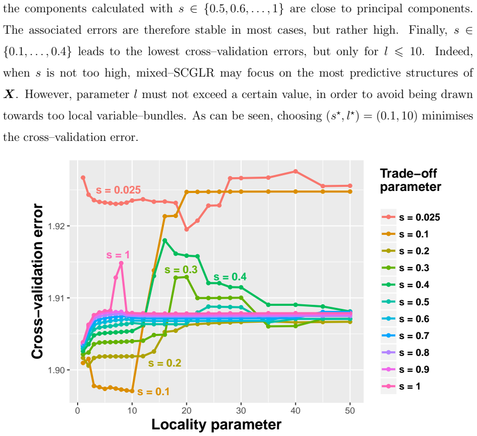
- The cross-validated locality parameter $l$ could itself be read as a diagnostic: small optimal $l$ indicates global principal-component-like structure, large $l$ indicates local bundles, so tuning doubles as an exploratory tool.
- In the $p>n$ simulations the number of components kept is a stronger regularisation choice than in the low-dimensional case; varying $K$ jointly with the principal-component cutoff would reveal how much of the method's performance hinges on that choice.
Signed reviews
Editorial analysis
A structured set of objections, weighed in public.
Referee Report
Summary. The paper extends Supervised Component-based Generalised Linear Regression (SCGLR) to multivariate generalized linear mixed models for grouped data. The proposed mixed-SCGLR method models q responses with linear predictors η_k = (Xu)γ_k + Aδ_k + Uξ_k, where X contains many redundant predictors, A contains few covariates of interest, and U is the random-effects design matrix. Estimation alternates between: (i) computing supervised components by maximizing a criterion that combines structural relevance and the goodness-of-fit of Schall's linearised working variables; (ii) solving Henderson systems for fixed effects, random effects, and variance components; and (iii) updating working variables and weights. Higher-rank components are extracted under orthogonality constraints via the PING algorithm. The method is evaluated on extensive simulations with Gaussian, Bernoulli, Poisson, and binomial outcomes, on high-dimensional settings, and on a forest ecology dataset with 22 concessions, and is compared with ridge and LASSO regularisations. The main claims are that mixed-SCGLR yields accurate fixed-effect estimates and interpretable components for grouped data, and that accounting for within-group dependence improves prediction over SCGLR.
Significance. The problem addressed is practically important: regularised regression for non-independent grouped data with many redundant predictors is common in ecology, epidemiology, and social science. If the central claims hold, mixed-SCGLR is a useful addition to the toolbox, especially because it provides interpretable supervised components in a GLMM setting where L1/L2 penalised methods are less interpretable. The paper's strengths include a clearly specified algorithm, extensive simulations covering several response distributions and high-dimensional cases, a real-data application, and the release of R code and a package. The PING algorithm is given in supplementary material. The main caveat is that the component criterion uses Schall working variables that contain the random-effects term, and no mechanism guarantees that this term does not influence the selected component directions. This issue is addressable and the central idea is defensible, so the paper merits revision rather than rejection.
major comments (3)
- [Section 4.1.2, Eq. (10) and Algorithm 1 Step 1] The goodness-of-fit criterion ψ_A(u) projects the working variable z^ξ_k, which satisfies z^ξ_k = (Xu)γ_k + Aδ_k + Uξ_k + e_k, onto span{Xu,A} using the conditional metric W^ξ_k. The marginal covariance of z^ξ_k is W^{ξ-1}_k + U D_k U^T, not W^{ξ-1}_k. Unless U^T W^ξ_k X u = 0 and U^T W^ξ_k A = 0, which the model does not imply, the random-effect term Uξ_k contributes to the projection and this contribution depends on u. Consequently, the component selected by (10) can be aligned with group-level variation rather than with the fixed structural relationship, and this potential contamination is inherited by the Henderson-system estimates in Step 2. The Gaussian simulations in Section 5.1 generate X independently of ξ, which may understate the problem; the real-data setting in Section 6, with plots grouped into 22 concessions, is exactly a setting where group-level confounding is plausible. Please address this by either modifying the criterion, for example by using the marginal covariance of the working variable or by projecting out the random-effect subspace, or by providing additional simulations in which X has group structure or is correlated with the random effects, together with a discussion of the sensitivity of the fixed-effect estimates.
- [Section 5.3, Tables 2 and 3] The simulation comparisons report only point estimates of MURSE and MRSE over B=100 samples, with no standard errors, confidence intervals, or Monte Carlo error estimates. Some of the reported differences are small relative to what one would expect from 100 replications; for example, Table 2 shows MURSE 0.10 for mixed-SCGLR versus 0.13 for LMM-ridge at τ=0.3, and Table 3 shows a Poisson MRSE of 0.30 for GLMM-LASSO versus 0.46 for mixed-SCGLR at τ=0.1. The same issue affects the supplementary tables. Since the ordering claims are central to the paper's conclusions, please add Monte Carlo standard errors or confidence intervals for the main comparisons, or at least for the entries that support the claimed ordering.
- [Section 4.2, Algorithm 1] No convergence guarantee or detailed convergence diagnostics are provided for the alternating algorithm. The stopping rule is described as iteration 'until stability of parameters is reached', but the tolerance, the maximum number of iterations, and the failure rate across the B=100 simulation replications are not reported. Section 6.2 notes non-convergence for s=0, which indicates that convergence behaviour is not automatic. Because the method's output, and hence the accuracy and interpretation claims, depends on this iteration, please add empirical convergence diagnostics (for example, the number of runs that reached the stated tolerance and the distribution of the number of iterations) and, if possible, a local convergence argument for the combined criterion maximised in Step 1.
minor comments (6)
- [Algorithm 1, Step 2] In the displayed Henderson system of Algorithm 1, the off-diagonal blocks involving A^T W f and U^T W f use f^{[t]} while the first row and the diagonal blocks use f^{[t+1]}; this is presumably a typo and should use f^{[t+1]} consistently throughout the matrix.
- [Section 4.1.2, Eq. (10)] The notation in Eq. (10) omits the iteration index [t] that is used elsewhere in Algorithm 1; adding these superscripts would make the dependence of ψ_A on the current working variables and weights explicit and easier to check.
- [Section 7] The acknowledged bias toward zero of variance-component estimates for binary outcomes should be connected to the role of D_k in Algorithm 1. Since D_k enters the Henderson system and the variance-component update, an underestimated σ_k^2 will affect the next iteration's working variables and weights; a brief discussion of this propagation, or a diagnostic in the Bernoulli simulations, would help the reader judge the practical impact.
- [Section 5.2 and supplementary material] The cross-validation procedure is described as 'leave-two-observations-out per group' with five parts, but the paper does not report the variability of the selected tuning parameters s*, K*, and λ* across the 100 samples; reporting, for example, the observed range of K* and the standard deviation of s* would strengthen the calibration discussion.
- [References] The reference to Bry et al. (2018) is given as 'In press'; if the paper has since been published, please update the citation with the journal, volume, and pages.
- [Figure 3] Figure 3 contains many overlapping curves and is difficult to read, especially for intermediate values of s; a small multiple of panels or a heatmap of the cross-validation error over the (s,l) grid would be clearer.
Circularity Check
No significant circularity: the component criterion, parameter updates, and cross-validated comparisons are all defined independently of the reported predictions.
full rationale
The paper's derivation chain is self-contained in the sense required by the circularity pass. The supervised component criterion (Eq. 10) is a goodness-of-fit measure built from the Schall-linearised working variables z^ξ_k defined in Eq. (9), with the random-effects design term Uξ_k included in the linearised model; the component u is then obtained by maximising a weighted combination of this criterion with a structural-relevance index φ(u) that depends only on X. No target quantity (fixed-effect estimate, cross-validation error, or variance component) is used to define the criterion, and no fitted constant is later reported as a prediction. Tuning parameters (K, s, l, ridge/LASSO shrinkage) are selected by out-of-sample 5-fold cross-validation in Sections 5.2 and 6.2, so the comparative claims in Tables 2, 3 and 4 are not forced by construction. The authors' own Section 7 limitation that binary-data variance components can be biased toward zero is an acknowledged inferential weakness of Schall's linearisation, not a circular step; likewise, the concern that the working criterion projects Uξ_k onto the component space is a statistical bias or confounding issue, not an equation-level reduction. The self-citations to Bry et al. (2013, 2018) justify the SCGLR criterion and a linear-algebra fact about loading vectors, but the mixed-model extension, the algorithm, the simulations, and the real-data comparison stand independently of those citations. Accordingly, no load-bearing step reduces to its own input.
Assumptions & free parameters
free parameters (3)
- s (trade-off between structural relevance and goodness-of-fit) =
cross-validated (e.g., 0.1 on the real data)
- l (bundle locality parameter) =
4 in the main simulations, 10 on the real data
- K (number of components) =
15 to 2 across simulations, 4 on the real data
assumptions (6)
- domain assumption Responses are independent conditional on the components and random effects.
- domain assumption Random effects are normally distributed with variance D_k = sigma^2_k I_N.
- domain assumption Schall's linearisation (PQL-type approximation) yields a valid working model for the GLMM.
- ad hoc to paper The structural-relevance criterion phi with a chosen l identifies the latent bundles in X.
- ad hoc to paper PING converges to a local maximum of the component criterion.
- domain assumption Replacing X by its principal components C preserves the structurally relevant information for high-dimensional data.
Cite this review
Pith. "Pith review of Component-based regularisation of multivariate generalised linear mixed models." pith.science (2026). https://pith.science/paper/5HKLMUB4
@misc{pith2026190804020,
  author       = {Pith},
  title        = {Pith review of: Component-based regularisation of multivariate generalised linear mixed models},
  year         = {2026},
  howpublished = {\url{https://pith.science/paper/5HKLMUB4}},
  note         = {Machine review of arXiv:1908.04020}
}
read the original abstract
We address the component-based regularisation of a multivariate Generalised Linear Mixed Model (GLMM) in the framework of grouped data. A set Y of random responses is modelled with a multivariate GLMM, based on a set X of explanatory variables, a set A of additional explanatory variables, and random effects to introduce the within-group dependence of observations. Variables in X are assumed many and redundant so that regression demands regularisation. This is not the case for A, which contains few and selected variables. Regularisation is performed building an appropriate number of orthogonal components that both contribute to model Y and capture relevant structural information in X. To estimate the model, we propose to maximise a criterion specific to the Supervised Component-based Generalised Linear Regression (SCGLR) within an adaptation of Schall's algorithm. This extension of SCGLR is tested on both simulated and real grouped data, and compared to ridge and LASSO regularisations. Supplementary material for this article is available online.
Figures
Figures from the paper (7 more)


Reference graph
Works this paper leans on
-
[1]
Anderson, D. A. and Aitkin, M. (1985). Variance C omponent M odels with B inary R esponse: I nterviewer V ariability. Journal of the Royal Statistical Society, Series B (Methodological) , 47(2):203--210
work page 1985
-
[2]
Bates, D., M \"a chler, M., Bolker, B., and Walker, S. (2015). Fitting linear mixed-effects models using lme4 . Journal of Statistical Software , 67(1):1--48
2015
-
[3]
Breslow, N. E. and Clayton, D. G. (1993). Approximate I nference in G eneralized L inear M ixed M odels. Journal of the American Statistical Association , 88(421):9--25
work page 1993
-
[4]
Bry, X., Trottier, C., Mortier, F., and Cornu, G. (2018). Component-based regularisation of a multivariate GLM with a thematic partitioning of the explanatory variables . Statistical Modelling . In press
work page 2018
-
[5]
Bry, X., Trottier, C., Mortier, F., Cornu, G., and Verron, T. (2014). Extending SCGLR to multiple regressor-groups: The T heme- SCGLR method. In Proceedings of the eighth International Conference on Partial Least Squares and Related Methods , Paris, France
work page 2014
-
[6]
Bry, X., Trottier, C., Mortier, F., Cornu, G., and Verron, T. (2016). The Multiple Facets of Partial Least Squares and Related Methods , chapter Supervised C omponent G eneralized L inear R egression with M ultiple E xplanatory B locks: THEME-SCGLR , pages 141--154. Springer International Publishing
work page 2016
-
[7]
Bry, X., Trottier, C., Verron, T., and Mortier, F. (2013). Supervised component generalized linear regression using a PLS -extension of the F isher scoring algorithm. Journal of Multivariate Analysis , 119(4):47--60
work page 2013
-
[8]
Bry, X. and Verron, T. (2015). THEME : THE matic M odel E xploration through multiple co-structure maximization. Journal of Chemometrics , 29(12):637--647
work page 2015
Show all 30 references
-
[9]
Clayton, D. G. (1996). Generalized linear mixed models. In Markov chain Monte Carlo in practice , pages 275--301. Springer
1996
-
[10]
Cornu, G., Mortier, F., Trottier, C., and Bry, X. (2018). SCGLR: Supervised Component Generalized Linear Regression . R package version 3.0
2018
-
[11]
P., and Foulkes, A
Eliot, M., Ferguson, J., Reilly, M. P., and Foulkes, A. S. (2011). Ridge R egression for L ongitudinal B iomarker D ata. The International Journal of Biostatistics , 7(1):1--11
2011
-
[12]
and Tutz, G
Fahrmeir, L. and Tutz, G. (1994). Multivariate Statistical Modelling Based on Generalized Linear Models . Springer Series in Statistics. Springer-Verlag
1994
-
[13]
Groll, A. (2017). glmmLasso: Variable Selection for Generalized Linear Mixed Models by L1-Penalized Estimation . R package version 1.5.1
2017
-
[14]
and Tutz, G
Groll, A. and Tutz, G. (2014). Variable s election for g eneralized l inear m ixed m odels by L _1 - p enalized e stimation. Statistics and Computing , 24(2):137--154
2014
-
[15]
Hadfield, J. D. (2010). MCMC M ethods for M ulti- R esponse G eneralized L inear M ixed M odels: the MCMC glmm R P ackage. Journal of Statistical Software , 33(2):1--22
2010
-
[16]
Henderson, C. R. (1975). Best L inear U nbiased E stimation and P rediction under a S election M odel. Biometrics , 31(2):423--447
1975
-
[17]
Hoerl, A. E. and Kennard, R. W. (1970). Ridge R egression: Biased E stimation for N onorthogonal P roblems. Technometrics , 12(1):55--67
1970
-
[18]
Knudson, C. (2016). Monte C arlo L ikelihood A pproximation for G eneralized L inear M ixed M odels . PhD thesis, University of Minnesota
2016
-
[19]
and Nelder, J
McCullagh, P. and Nelder, J. (1989). Generalized Linear Models, Second Edition . Chapman & Hall/CRC Monographs on Statistics & Applied Probability. Taylor & Francis
1989
-
[20]
McCulloch, C. E. (1997). Maximum L ikelihood A lgorithms for G eneralized L inear M ixed M odels. Journal of the American Statistical Association , 92(437):162--170
1997
-
[21]
Nelder, J. A. and Wedderburn, R. W. M. (1972). Generalized L inear M odels. Journal of the Royal Statistical Society. Series A (General) , 135(3):370--384
1972
-
[22]
Pinheiro, J. C. and Bates, D. M. (1995). Approximations to the L og- L ikelihood F unction in the N onlinear M ixed- E ffects M odel. Journal of Computational and Graphical Statistics , 4(1):12--35
1995
-
[23]
R: A Language and Environment for Statistical Computing
R Core Team (2017). R: A Language and Environment for Statistical Computing . R Foundation for Statistical Computing, Vienna, Austria
2017
-
[24]
Schall, R. (1991). Estimation in G eneralized L inear M odels with R andom E ffects. Biometrika , 78(4):719--727
1991
-
[25]
Schelldorfer, J., Meier, L., and B \"u hlmann, P. (2014). GLMMLasso : An A lgorithm for H igh- D imensional G eneralized L inear M ixed L odels U sing _1 - P enalization. Journal of Computational and Graphical Statistics , 23(2):460--477
2014
-
[26]
and McCullagh, P
Shun, Z. and McCullagh, P. (1995). Laplace A pproximation of H igh D imensional I ntegrals. Journal of the Royal Statistical Society, Series B (Methodological) , 57(4):749--760
1995
-
[27]
Tibshirani, R. (1996). Regression S hrinkage and S election via the L asso. Journal of the Royal Statistical Society, Series B (Methodological) , 58(1):267--288
1996
-
[28]
Zeger, S. L. and Karim, M. R. (1991). Generalized L inear M odels W ith R andom E ffects; A G ibbs S ampling A pproach. Journal of the American Statistical Association , 86(413):79--86
1991
-
[29]
Zhang, Y., Zhou, H., Zhou, J., and Sun, W. (2017). Regression M odels for M ultivariate C ount D ata. Journal of Computational and Graphical Statistics , 26(1):1--13
2017
-
[30]
and Hastie, T
Zou, H. and Hastie, T. (2005). Regularization and variable selection via the elastic net. Journal of the Royal Statistical Society, Series B (Methodological) , 67(2):301--320
2005
Reviewed August 14, 2026 · model on record in the stance chip above.
Discussion (0). Continue with ORCID to comment.