Maximum Approximated Likelihood Estimation

Constantin Weiser; Florian Heiss; Jens Oettershagen; Michael Griebel

REVIEW 3 major objections 5 minor 33 references

Maximum Approximated Likelihood Estimation

T0 review · 3 major / 5 minor · reviewed 2026-08-14 · deepseek-v4-flash

Challenge this review Re-run · record.json Download PDF Read on arXiv ↗ Review JSON

Pith's one-line read This paper proves that maximum approximated likelihood estimators have the same asymptotic distribution as exact maximum likelihood whenever the approximation's worst-case error, including the gradient, shrinks faster than $n^{-1/2}$.

desk verdict A clean maximal-approximated-likelihood framework whose central theorems require uniform approximation error over the whole covariate space, a condition the paper's own mixed-logit example with unbounded covariates fails, so the examples outrun the theorems as stated. read the letter →

arxiv 1908.04110 v1 pith:UI4TMIDO submitted 2019-08-12 econ.EM math.STstat.TH

Michael Griebel , Florian Heiss , Jens Oettershagen , Constantin Weiser This is my paper · ORCID

classification econ.EMmath.STstat.TH MSC 62F1262E2065D30

keywords maximumapproximatedlikelihoodsimulatedquadraturequasi-MonteCarlosparsegridsasymptoticnormalitymixedlogitnumericalintegration

verification ladder T0 review T1 audit T2 compute T3 formal

The pith

A machine-rendered reading of the paper's core claim, the machinery that carries it, and where it could break.

The reading

The paper asks whether replacing an intractable likelihood by a numerical approximation—a quadrature rule, quasi-Monte Carlo points, or a sparse grid—changes the statistical conclusions. Its answer is that the approximation error is asymptotically irrelevant precisely when the worst-case error, measured jointly on the likelihood and its gradient, disappears faster than $1/\sqrt{n}$ as the number of integration points grows with the sample size. Under that condition the maximum approximated likelihood estimator is consistent and asymptotically normal with the same covariance matrix as the infeasible maximum likelihood estimator. The paper also translates the condition into growth requirements for the number of integration points, and shows that exponentially convergent rules need only logarithmically many points, in contrast to Monte Carlo simulation which needs roughly as many points as observations. This matters for applied work because many discrete-choice and random-effects models have likelihoods defined by integrals that cannot be computed in closed form.

What carries the argument

The central object is the worst-case approximation error $E(r)$ defined in equation (3.7), together with the link function $R:\mathbb{N}\to\mathbb{N}$ that couples the number of integration points to the sample size. The proof route is to view $\hat\theta_{\mathrm{MAL}}$ as an extremum estimator with an approximated objective and transfer uniform convergence of the approximation to the log-likelihood and its first two derivatives; a technical lemma on logarithms bounds the distance between $\log\tilde f$ and $\log f$ by a multiple of the distance between $\tilde f$ and $f$, provided each is bounded away from zero. What carries the argument is that the condition $\sqrt{n}E(R(n))\to 0$ is the natural rate threshold: it makes the approximation error in the score negligible against the $O_p(n^{-1/2})$ size of the exact score.

What would settle it

Take a model with a known true parameter and approximate the likelihood by Monte Carlo with $r=n^\beta$ for $\beta=1/2$ and $\beta=1$. The theorem predicts that the second estimator is asymptotically normal with variance $I^{-1}$, while the first uses a link function for which $\sqrt{n}E(R(n))$ does not vanish; a simulation showing the opposite would refute the claimed rate threshold. A sharper check is to compute the actual worst-case error $E(R(n))$ for a Gauss-Hermite approximation of a mixed-logit likelihood with bounded covariates and verify numerically whether $\sqrt{n}E(R(n))$ tends to zero under the prescribed $R(n)$ while the estimator's distribution matches $N(0,I^{-1})$.

Watch

Extended reading notes

Core claim

The central claim is that maximum approximated likelihood (MAL) estimation inherits the statistical properties of maximum likelihood once the approximation is good enough relative to the sample size. Define $E(r)=\sup_{z\in\mathcal{Z},\theta\in\Theta}(|\tilde f_r(z,\theta)-f(z,\theta)|+\|\nabla_\theta \tilde f_r(z,\theta)-\nabla_\theta f(z,\theta)\|)$. If $R(n)$ quadrature points are used for a sample of size $n$, and $\sqrt{n}E(R(n))\to 0$ in probability, then $\sqrt{n}(\hat\theta_{\mathrm{MAL}}-\theta_0)\xrightarrow{d} N(0,I^{-1})$, the same limit the exact maximum likelihood estimator would have. The paper proves this by treating the approximated log-likelihood as an M-estimator objective and showing that the approximation error in the gradient is controlled by $E(R(n))$; the same argument gives consistency from uniform convergence of $\tilde f_{R(n)}$ to $f$. Rate conclusions follow: algebraic convergence $E(r)\le cr^{-s}$ requires $R(n)\sim n^{\gamma/s}$ for any $\gamma>1/2$, while exponential convergence $E(r)\le c e^{-\alpha r^\beta}$ requires only $R(n)\sim(\log n)^{1/\beta}$.

Load-bearing premise

The whole argument hangs on the assumption that the approximation error has a finite worst case over every possible data point and every parameter value, and that this worst case shrinks uniformly; with unbounded covariates this is not available for the mixed-logit example, because derivatives of the logit grow linearly in the covariate.

Editorial extensions

If this is right

For deterministic rules with exponential convergence, $R(n)$ as small as $(\log n)^{1/\beta}$ suffices, so the computational cost is roughly $n\log n$ integrand evaluations instead of $n^2$ for Monte Carlo under identical sampling.
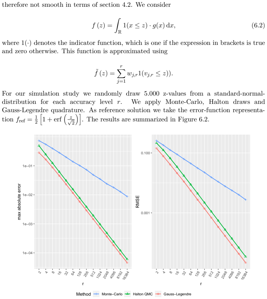
Quasi-Monte Carlo rules with error $O(r^{-1+\varepsilon})$ require $R(n)=n^\beta$ with $\beta>1/2$, a square-root reduction compared with Monte Carlo.
Gaussian quadrature and sparse-grid approximations can therefore deliver estimators with the same asymptotic efficiency as exact maximum likelihood at substantially lower cost, provided the integrand has the required smoothness.
The paper's conditions also imply a practical warning: for a fixed approximation accuracy, the extra estimation error grows with the sample size, so large datasets demand more accurate quadrature than small ones.

Reading between the lines

Editorial extensions of the paper, not claims the author makes directly.

The sup-norm formulation suggests a testable modification: replacing the supremum over an unbounded data space by an expectation-weighted norm might extend the theorem to mixed-logit settings with unbounded covariates, where the current worst-case condition is infinite.
The framework likely transfers to other approximate M-estimators such as simulated GMM or minimum distance, since the underlying argument only uses uniform convergence of the approximated objective and its derivatives.
The rate threshold suggests an adaptive implementation: a practitioner could estimate the quadrature error and keep increasing $r$ until the error is below $c/\sqrt{n}$, instead of committing to a fixed link function.
The finite-sample simulations imply that efficiency comparisons among approximation methods can be made before fitting the model, by checking which rule has the smaller worst-case error at the chosen $R(n)$.

Share X Bluesky LinkedIn Reddit HN

Signed reviews

No signed human review yet.

Editorial analysis

A structured set of objections, weighed in public.

Desk editor's note, referee report, and a circularity audit.

Desk Editor's Note

read the letter

Dear Colleague,

This is a useful paper and the core is right, but the headline examples outrun the theorems. What's genuinely new: a general MAL framework where consistency and asymptotic normality are expressed through a single worst-case approximation error E(r) that includes the function and its gradient. That is a clean abstraction. It nests MSL as a special case and gives explicit link functions R(n) for Monte Carlo, QMC, Gaussian quadrature, and sparse grids. The algebra in Theorem 9 is correct, and the simulation study is honest and well matched to the theory.

The soft spot is real and located in the scope conditions. Theorem 7 requires f ≥ δ > 0 on all of Z×Θ, and Theorem 8 requires E(r) = sup_{z∈Z, θ∈Θ} |\tilde f_r − f| + ||∇\tilde f_r − ∇f|| to go to zero uniformly. Those are strong. In the paper's own mixed-logit example (Example Ia), Z = R. For fixed r, as z → ∞ the true f tends to 1 while the Gauss–Hermite approximation converges to W_r(θ), the total weight of nodes above a threshold, which is generically not 1. So sup_z |\tilde f_r − f| ≥ |1 − W_r(θ)| > 0 for every finite r. The gradient term is worse: its z-dependence makes the supremum infinite. The verification in Section 5 only checks smoothness of the integrand in v, not uniformity over z. So as stated, the theorems do not cover the motivating example. The proof of Theorem 8 also silently uses sup_{z,θ} ||∇f|| and sup_{z,θ} ||∇θθ f|| to define C1 and C2; those need to be finite, which again fails for unbounded covariates.

This is not a contradiction inside the theorems—they are true under the stated conditions—it is a missing scope condition. The fix is straightforward: either assume Z is bounded (or covariates have compact support), or replace the sup-norm with a weighted sup-norm or an L_p(μ) norm under the data distribution, which is what the log-likelihood average actually needs. Kristensen and Salanié (2017) is a related reference for exactly this kind of relaxation.

Who is this for? Anyone working on theory for approximated likelihood estimators, and practitioners who want to know when deterministic quadrature is asymptotically safe. I would send it to a serious referee; the framework deserves to be in the literature, but it needs the scope conditions stated honestly before it can serve as blanket justification for deterministic quadrature.

Recommendation: engage with it, but tell the authors to fix the sup-norm gap before publication.

Referee Report

3 major / 5 minor

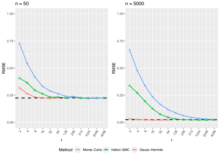
Summary. The paper develops asymptotic theory for maximum approximated likelihood (MAL) estimators, in which each log-likelihood contribution is replaced by a numerical quadrature approximation with an accuracy level r that grows with the sample size n. It states general consistency and asymptotic normality results for MAL estimators (Theorems 7 and 8), derives sufficient growth rates for r under algebraic and exponential quadrature error bounds (Theorem 9), and applies the framework to Monte Carlo, quasi-Monte Carlo, Gauss-Hermite quadrature, and sparse grid integration. The theoretical results are illustrated with mixed logit and Butler-Moffitt examples and a simulation study comparing approximation methods.

Significance. If the stated conditions are met, the paper gives a useful unifying framework: maximum simulated likelihood emerges as a special case, and the link-function results (e.g., logarithmic growth of r for exponentially convergent quadrature) are practically relevant. The algebraic manipulations in Theorem 9 are correct, and the proofs of the general theorems follow standard extremum-estimator arguments. The paper also provides a helpful simulation comparison of approximation methods. However, the scope of the central theorems is narrower than the examples suggest: the uniform sup-norm error condition used throughout is not satisfied for the paper's own mixed logit examples when covariates are unbounded, which is the standard empirical setting. This gap is load-bearing and requires a substantial clarification or modification of the assumptions.

major comments (3)

[Section 5, Example Ia; Theorem 7(iii) and Eq. (3.7)] For the mixed logit example with unbounded covariates, the uniform approximation error E(r)=sup_{z∈Z,θ∈Θ}(|\tilde f_r(z,θ)-f(z,θ)|+||∇_θ \tilde f_r(z,θ)-∇_θ f(z,θ)||) does not vanish as r→∞. With f(z,θ)=∫ σ(z(θ2 v+θ1)) φ(v) dv and Gauss-Hermite quadrature, for fixed r and z→∞, \tilde f_r(z,θ) tends to W_r(θ)=Σ_{j: θ2 v_j+θ1>0} w_j while f(z,θ)→1, so sup_z |\tilde f_r-f| is bounded below by a positive constant for generic θ. The gradient term is worse: ∂\tilde f_r/∂θ1=Σ_j w_j z σ'(z(θ2 v_j+θ1)) has no finite supremum over z∈R when θ2 v_j+θ1=0 for some node, and over a compact parameter set containing points arbitrarily close to such a hyperplane the supremum is unbounded. Thus Theorem 7(iii) and Theorem 8(ii) fail for the paper's headline example unless Z is assumed bounded or the error norm is changed to a data-dependent or weighted norm. This is a missing scope condition, not a contradiction inside the theorems, but it must be addressed for the examples to be covered by the theory.
[Proof of Theorem 8, constants C1(f) and C2(f)] The proof of Theorem 8 defines C1(f) and C2(f) using sup_{z∈Z,θ∈Θ}||∇_θ f(z,θ)|| and sup_{z∈Z,θ∈Θ}||∇_{θθ} f(z,θ)||, and then bounds the approximation error of the log-likelihood gradient by C1(f)√n E(R(n)). However, the assumptions of Theorem 8 do not state that these suprema are finite. If Z is unbounded, as in the mixed logit example, the suprema are infinite, and the displayed inequality is not justified. The proof therefore implicitly assumes uniform boundedness of f and its θ-derivatives up to order two over Z×Θ; this assumption needs to be stated explicitly and verified in the applications.
[Section 5 and Lemma 20] The verification of the Gauss-Hermite error bounds for the logit examples is incomplete. Lemma 20 provides bounds of the form |D^{(θ)}_α D^{(v)}_β f(θ,v)| ≤ c(α,β) θ^β e^{v^T v/2} ∏ sqrt(1+v_i^2), so the constant depends on the parameter θ through the factor θ^β. When applied to φ(v,z_i,θ)=σ(z_i(θ2 v+θ1)), the relevant parameter vector includes z_i, so the constant c(k,α) is actually a function of z_i and is not uniform over an unbounded covariate space Z. Consequently, the paper does not establish the uniform-in-z bound (4.10) or (4.13) that is needed to obtain a finite, r-independent constant in the quadrature error estimate (4.11) for the mixed logit example.

minor comments (5)

[Theorem 2] The conclusion of Theorem 2 states 'plim_{n→∞} \hatθ_M = θ0'; this should refer to the approximated estimator \hatθ_AM, not the infeasible M-estimator \hatθ_M.
[Section 2, after Theorem 2] The sentence beginning 'accuracy parameter r to the number of observations n we introduce a function R' lacks a subject or transition; it should read something like 'To link the accuracy parameter r to the number of observations n, we introduce a function R: N→N.'
[Corollary 11] The condition numbering in Corollary 11 jumps from (ii) to (iv); condition (iii) is missing.
[Section 6, Figure 6.3] The vertical axis of Figure 6.3 is labeled 'n × max abs Err', but the text and the caption refer to √n E(R(n)); the label should be √n × max abs Err to match the quantity being plotted.
[Section 1, paragraph 2] The word 'independed' should be 'independent'.

Circularity Check

0 steps flagged · score 0.0 of 10

No significant circularity: the paper proves conditional asymptotic theorems from standard extremum-estimator arguments and cites external quadrature-error bounds; no prediction reduces to a fitted input or self-citation by construction.

full rationale

This paper's results are conditional asymptotic theorems. Theorems 2 and 4 show that an extremum estimator based on a uniformly consistent approximation of the objective function inherits consistency and asymptotic normality; both proofs proceed directly from Newey-McFadden-type arguments via the triangle inequality and do not use the target result as an input. Theorem 8 makes the required rate explicit by defining E(r) as the worst-case error in the approximated likelihood and its gradient, then proves that the condition sqrt(n) E(R(n)) -> 0 is sufficient for the MAL estimator to have the same limit distribution as the infeasible MLE; the conclusion is a proof that this condition suffices, not a claim that any particular approximation scheme satisfies it. Theorem 9 converts assumed algebraic or exponential error bounds into a required growth rate R(n); the derivation is simple algebra and contains no fitted parameters. The self-citations (Griebel and Oettershagen; Gerstner and Griebel) are used only as sources for sparse-grid and tensor-product error estimates, which are independent numerical-analysis statements about quadrature rules and do not presuppose the paper's econometric conclusions. No parameter is estimated from the target data, no uniqueness theorem is imported from the authors' own prior work to exclude alternatives, and no known empirical pattern is renamed as a theoretical result. The applied examples inherit assumptions from external quadrature-error theorems; whether those assumptions hold for unbounded covariate spaces is a scope or correctness question, not a circularity. The paper is therefore self-contained against external benchmarks for the claims it actually states.

Assumptions & free parameters 0 free parameters · 6 assumptions · 0 invented entities

The central theorems rest on the standard Newey-McFadden regularity conditions for the exact MLE, on a uniform positive lower bound for the likelihood contributions, on uniform sup-norm convergence of the quadrature approximations over Z x Theta, and on external numerical analysis error bounds. No free parameters are fitted and no new entities are postulated. The most fragile requirement is uniform boundedness of the likelihood and its derivatives over the whole data space, which is implicit in the proof of Theorem 8 and absent from the stated assumptions.

assumptions (6)

domain assumption The infeasible ML estimator satisfies the standard Newey-McFadden regularity conditions (compact parameter space, identification, dominance) for consistency and asymptotic normality.
Assumed in Lemmas 5 and 6 and carried into Theorems 7 and 8; the paper abstracts from misspecification to focus on approximation error.
domain assumption The likelihood contributions f(z,theta) are bounded below uniformly by delta > 0 over z in Z, theta in Theta.
Theorem 7 condition (ii), needed to control log differences via 1/delta; strong for discrete choice models with extreme covariates or parameters.
domain assumption The quadrature rule converges uniformly over z in Z and theta in Theta for f, its gradient and Hessian (E(r), Ebar_k(r)).
Theorem 7(iii) and Theorem 8(ii)-(iii); requires uniform sup-norm convergence, not just pointwise or average convergence. For unbounded Z this may fail.
ad hoc to paper The functions f and its theta-derivatives up to order 2 are uniformly bounded over Z x Theta (needed for constants C1, C2 in the proof of Theorem 8).
Not stated explicitly as an assumption; implicitly used in the proof of Theorem 8 to define C1(f) and C2(f). Without it the bounds blow up.
standard math External quadrature error bounds (Gauss-Hermite, sparse grids, QMC) from cited numerical analysis literature hold in the required sup-norm form.
The paper relies on Smith et al. (1983), Gerstner and Griebel (1998), Zhang et al. (2013) and others for convergence rates; these are standard results but not re-derived.
ad hoc to paper For the logit examples, the integrand satisfies the growth conditions (4.10) or (4.13), verified via Lemma 20 assuming bounded covariates z.
Section 5 checks smoothness in v only; the bounds contain powers of z (through theta dot v), so uniform boundedness requires a compact data space, which is not stated.

how reviews work

0 comments

Cite this review

Pith. "Pith review of Maximum Approximated Likelihood Estimation." pith.science (2026). https://pith.science/paper/UI4TMIDO

@misc{pith2026190804110,
  author       = {Pith},
  title        = {Pith review of: Maximum Approximated Likelihood Estimation},
  year         = {2026},
  howpublished = {\url{https://pith.science/paper/UI4TMIDO}},
  note         = {Machine review of arXiv:1908.04110}
}

read the original abstract

Empirical economic research frequently applies maximum likelihood estimation in cases where the likelihood function is analytically intractable. Most of the theoretical literature focuses on maximum simulated likelihood (MSL) estimators, while empirical and simulation analyzes often find that alternative approximation methods such as quasi-Monte Carlo simulation, Gaussian quadrature, and integration on sparse grids behave considerably better numerically. This paper generalizes the theoretical results widely known for MSL estimators to a general set of maximum approximated likelihood (MAL) estimators. We provide general conditions for both the model and the approximation approach to ensure consistency and asymptotic normality. We also show specific examples and finite-sample simulation results.

Figures

Figures reproduced from arXiv: 1908.04110 by the authors.

**Figure 6.1.** Convergence behavior using different approximation methods for a smooth function f zi = (y, x), θ = β¯ = ´ R g(y − xβ) × g(β − β¯) dβ As shown in [PITH_FULL_IMAGE:figures/full_fig_p022_6_1.png] view at source ↗

**Figure 6.2.** Convergence behavior using different approximation methods for a non-smooth function f (z) = ´ R 1(x ≤ z) · g(x) dx The result for the non-smooth ARS confirms that the relative performance depends strongly 23 [PITH_FULL_IMAGE:figures/full_fig_p023_6_2.png] view at source ↗

**Figure 6.3.** Convergence of √ nE(R(n)) for different link functions on the smoothness of the approximated function. Here Monte-Carlo achieves the same convergence rate as before. The Halton draws and Gauss-Legendre achieve a higher rate, but Gauss-quadrature does not outperform the other two methods any more. As stated in section 3.2 the convergence rate of an approximation method translates into the required link-function R(n) … view at source ↗

Figures from the paper (2 more)

**Figure 6.4.** Figure 6.4: Convergence of the estimator with sample size n fixed Consequences for the practical application of MALE The overall estimation error (ˆθMAL −θ0) in MAL has two components (compare also equation (2.4)). First, the sampling error and, second, the approximation error.…

**Figure 6.** Figure 6: shows an increasing relevance of the approximation error due a rising number [PITH_FULL_IMAGE:figures/full_fig_p026_6.png]

Discussion (0). Continue with ORCID to comment.

Reference graph

Works this paper leans on

33 extracted references · 33 canonical work pages

[1]

Geweke, and J

Ackerberg, D., J. Geweke, and J. Hahn (2009) ‘Supplement to Comments on ”Convergence Properties of the Likelihood of Computed Dynamic Models”.’Econometrica77(6), 2009– 26 2017

work page 2009
[2]

(2001) ‘Quasi-random maximum simulated likelihood estimation of the mixed multinomial logit model.’Transportation Research Part B: Methodological35(7), 677– 693

Bhat, C. (2001) ‘Quasi-random maximum simulated likelihood estimation of the mixed multinomial logit model.’Transportation Research Part B: Methodological35(7), 677– 693

work page 2001
[3]

(1984) ‘Asymptotic coeﬃcients of Hermite function series.’J

Boyd, J. (1984) ‘Asymptotic coeﬃcients of Hermite function series.’J. of Computational Physics pp. 382–410

work page 1984
[4]

Moﬃtt (1982) ‘A computationally eﬃcient quadrature procedure for the one factor multinomial probit model.’Econometrica50(3), 761–764

Butler, J., and R. Moﬃtt (1982) ‘A computationally eﬃcient quadrature procedure for the one factor multinomial probit model.’Econometrica50(3), 761–764

work page 1982
[5]

Rabinowitz (2007)Methods of Numerical IntegrationDover Books on Mathematics Series (Dover Publications)

Davis, P., and P. Rabinowitz (2007)Methods of Numerical IntegrationDover Books on Mathematics Series (Dover Publications)

work page 2007
[6]

Pillichshammer (2010)Digital Nets and Sequences

Dick, J., and F. Pillichshammer (2010)Digital Nets and Sequences. Discrepancy Theory and quasi-Monte Carlo Integration(Cambridge University Press, Cambridge)

work page 2010
[7]

Griebel (1998) ‘Numerical integration using sparse grids.’Numerical Algorithms 18, 209–232

Gerstner, T., and M. Griebel (1998) ‘Numerical integration using sparse grids.’Numerical Algorithms 18, 209–232

work page 1998
[8]

Griebel (2003) ‘Dimension–adaptive tensor–product quadrature.’ Computing 71(1), 65–87 Gouriéroux, C., and A

Gerstner, T., and M. Griebel (2003) ‘Dimension–adaptive tensor–product quadrature.’ Computing 71(1), 65–87 Gouriéroux, C., and A. Monfort (1996)Simulation-Based Econometric Methods(Oxford University Press)

work page 2003

Show all 33 references

[9]

Oettershagen (2014) ‘Dimension-adaptive sparse grid quadrature for in- tegrals with boundary singularities.’ In ‘Sparse grids and Applications,’ vol

Griebel, M., and J. Oettershagen (2014) ‘Dimension-adaptive sparse grid quadrature for in- tegrals with boundary singularities.’ In ‘Sparse grids and Applications,’ vol. 97 ofLecture Notes in Computational Science and Engineering(Springer) pp. 109–136 (2016) ‘On tensor product...

2014
[10]

McFadden (1998) ‘The method of simulated scores for the esti- mation of LDV models.’Econometrica66(4), 863–896

Hajivassiliou, V., and D. McFadden (1998) ‘The method of simulated scores for the esti- mation of LDV models.’Econometrica66(4), 863–896

1998
[11]

Ruud (1994) ‘Classical estimation methods for LDV models using simulation.’ In ‘Handbook of Econometrics,’ vol

Hajivassiliou, V., and P. Ruud (1994) ‘Classical estimation methods for LDV models using simulation.’ In ‘Handbook of Econometrics,’ vol. 4 pp. 2383–2441

1994
[12]

(1964) ‘Algorithm 247: Radical-inverse quasi-random point sequence.’Commun

Halton, J. (1964) ‘Algorithm 247: Radical-inverse quasi-random point sequence.’Commun. ACM 7(12), 701–702

1964
[13]

Winschel (2008) ‘Likelihood approximation by numerical integration on sparse grids.’J

Heiss, F., and V. Winschel (2008) ‘Likelihood approximation by numerical integration on sparse grids.’J. of Econometrics144(1), 62–80 27

2008
[14]

Train, and J

Hess, S., K. Train, and J. Polak (2006) ‘On the use of a modiﬁed Latin Hypercube Sam- pling (MLHS) method in the estimation of a Mixed Logit Model for vehicle choice.’ Transportation Research Part B: Methodological40(2), 147–163

2006
[15]

Markhasin, J

Hinrichs, A., L. Markhasin, J. Oettershagen, and T. Ullrich (2016) ‘Optimal quasi-Monte Carlo rules on higher order digital nets for the numerical integration of multivariate periodic functions.’Numerische Mathematik134(1), 163–196

2016
[16]

(1963) ‘On the method for numerical integration of Clenshaw and Curtis.’Nu- merische Mathematik5(1), 138–141

Imhof, J. (1963) ‘On the method for numerical integration of Clenshaw and Curtis.’Nu- merische Mathematik5(1), 138–141

1963
[17]

Kritzer, G

Irrgeher, C., P. Kritzer, G. Leobacher, and F. Pillichshammer (2015) ‘Integration in Her- mite spaces of analytic functions.’J. of Complexity31(3), 380–404

2015
[18]

Webster, and G

Jantsch, P., C. Webster, and G. Zhang (2016) ‘On the Lebesgue constant of weighted Leja points for Lagrange interpolation on unbounded domains.’ arXiv preprint arXiv:1606.07093

2016 arXiv
[19]

Kristensen, Dennis, and Bernard SalaniÃľ (2017) ‘Higher-order properties of approximate estimators.’Journal of Econometrics198(2), 189–208

2017
[20]

Woźniakowski (2011) ‘Gauss-Hermite quadratures for functions from Hilbert spaces with Gaussian reproducing kernels.’ BIT Numerical Mathematics 52(2), 425–436

Kuo, F., and H. Woźniakowski (2011) ‘Gauss-Hermite quadratures for functions from Hilbert spaces with Gaussian reproducing kernels.’ BIT Numerical Mathematics 52(2), 425–436

2011
[21]

Monegato (1994) ‘Error estimates for Gauss-Laguerre and Gauss- Hermite quadrature formulas.’ InApproximation and Computation: A Festschrift in Honor of Walter Gautschi,ed

Mastroianni, G., and G. Monegato (1994) ‘Error estimates for Gauss-Laguerre and Gauss- Hermite quadrature formulas.’ InApproximation and Computation: A Festschrift in Honor of Walter Gautschi,ed. R. Zahar, vol. 119 ofISNM International Series of Nu- merical Mathematics(Birkhae...

1994
[22]

(1989) ‘A method of simulated moments for estimation of discrete response models without numerical integration.’Econometrica57, 995–1026

McFadden, D. (1989) ‘A method of simulated moments for estimation of discrete response models without numerical integration.’Econometrica57, 995–1026

1989
[23]

Train (2000) ‘Mixed MNL models for discrete response.’J

McFadden, D., and K. Train (2000) ‘Mixed MNL models for discrete response.’J. of Applied Econometrics 15, 447–470

2000
[24]

McFadden (1994) ‘Large sample estimation and hypothesis testing.’ vol

Newey, W., and D. McFadden (1994) ‘Large sample estimation and hypothesis testing.’ vol. 4 pp. 2111–2245

1994
[25]

(1992) Random Number Generation and Quasi-Monte Carlo Methods (SIAM, Philadelphia)

Niederreiter, H. (1992) Random Number Generation and Quasi-Monte Carlo Methods (SIAM, Philadelphia)

1992
[26]

Ritter (1996) ‘High dimensional integration of smooth functions over cubes.’Numerische Mathematik75(1), 79–97 28

Novak, E., and K. Ritter (1996) ‘High dimensional integration of smooth functions over cubes.’Numerische Mathematik75(1), 79–97 28

1996
[27]

(2005) ‘Multidimensional variation for quasi-Monte Carlo.’ In ‘International Con- ference on Statistics in honour of Professor Kai-Tai Fang’s 65th birthday’ pp

Owen, A. (2005) ‘Multidimensional variation for quasi-Monte Carlo.’ In ‘International Con- ference on Statistics in honour of Professor Kai-Tai Fang’s 65th birthday’ pp. 49–74 (2006) ‘Halton sequences avoid the origin.’SIAM review48(3), 487–503

2005
[28]

Patterson, T.(1968)‘Theoptimumadditionofpointstoquadratureformulae.’ Mathematics of Computation22(104), 847–847 Sándor, Z., and K.Train(2004) ‘Quasi-randomsimulation ofdiscrete choicemodels.’Trans- portation Research Part B: Methodological38(4), 313 – 327

1968
[29]

Joe (1994)Lattice Methods for Multiple Integration(New York: Oxford University Press)

Sloan, I., and S. Joe (1994)Lattice Methods for Multiple Integration(New York: Oxford University Press)

1994
[30]

Sloan, and A

Smith, W., I. Sloan, and A. Opie (1983) ‘Product integration over inﬁnite intervals I . Rules based on the zeros of Hermite polynomials.’ 40(162), 519–535

1983
[31]

(1967) ‘The distribution of points in a cube and the approximate evaluation of integrals.’J

Sobol, I. (1967) ‘The distribution of points in a cube and the approximate evaluation of integrals.’J. Comp. Mathematics and Math. Physics7, 86–112

1967
[32]

(2009)Discrete Choice Methods with Simulation,2nd ed

Train, K. (2009)Discrete Choice Methods with Simulation,2nd ed. (Cambridge University Press)

2009
[33]

Gunzburger, and W

Zhang, G., M. Gunzburger, and W. Zhao (2013) ‘A sparse grid method for multi- dimensional backward stochastic diﬀerential equations.’J. of Computational Mathemat- ics 31(3), 221–248 A. Appendix: Technical results In Section 3, we have worked with distances of the log likelihoo...

2013

Pith tools

Reviewed August 14, 2026 · model on record in the stance chip above.

[1] [1]

Geweke, and J

Ackerberg, D., J. Geweke, and J. Hahn (2009) ‘Supplement to Comments on ”Convergence Properties of the Likelihood of Computed Dynamic Models”.’Econometrica77(6), 2009– 26 2017

work page 2009

[2] [2]

(2001) ‘Quasi-random maximum simulated likelihood estimation of the mixed multinomial logit model.’Transportation Research Part B: Methodological35(7), 677– 693

Bhat, C. (2001) ‘Quasi-random maximum simulated likelihood estimation of the mixed multinomial logit model.’Transportation Research Part B: Methodological35(7), 677– 693

work page 2001

[3] [3]

(1984) ‘Asymptotic coeﬃcients of Hermite function series.’J

Boyd, J. (1984) ‘Asymptotic coeﬃcients of Hermite function series.’J. of Computational Physics pp. 382–410

work page 1984

[4] [4]

Moﬃtt (1982) ‘A computationally eﬃcient quadrature procedure for the one factor multinomial probit model.’Econometrica50(3), 761–764

Butler, J., and R. Moﬃtt (1982) ‘A computationally eﬃcient quadrature procedure for the one factor multinomial probit model.’Econometrica50(3), 761–764

work page 1982

[5] [5]

Rabinowitz (2007)Methods of Numerical IntegrationDover Books on Mathematics Series (Dover Publications)

Davis, P., and P. Rabinowitz (2007)Methods of Numerical IntegrationDover Books on Mathematics Series (Dover Publications)

work page 2007

[6] [6]

Pillichshammer (2010)Digital Nets and Sequences

Dick, J., and F. Pillichshammer (2010)Digital Nets and Sequences. Discrepancy Theory and quasi-Monte Carlo Integration(Cambridge University Press, Cambridge)

work page 2010

[7] [7]

Griebel (1998) ‘Numerical integration using sparse grids.’Numerical Algorithms 18, 209–232

Gerstner, T., and M. Griebel (1998) ‘Numerical integration using sparse grids.’Numerical Algorithms 18, 209–232

work page 1998

[8] [8]

Griebel (2003) ‘Dimension–adaptive tensor–product quadrature.’ Computing 71(1), 65–87 Gouriéroux, C., and A

Gerstner, T., and M. Griebel (2003) ‘Dimension–adaptive tensor–product quadrature.’ Computing 71(1), 65–87 Gouriéroux, C., and A. Monfort (1996)Simulation-Based Econometric Methods(Oxford University Press)

work page 2003