Mixture-based Multiple Imputation Model for Clinical Data with a Temporal Dimension

Diego Klabjan; Ye Xue; Yuan Luo

REVIEW 3 major objections 4 minor 72 references

Mixture-based Multiple Imputation Model for Clinical Data with a Temporal Dimension

T0 review · 3 major / 4 minor · reviewed 2026-08-14 · deepseek-v4-flash

Challenge this review Re-run · record.json Download PDF Read on arXiv ↗ Review JSON

Pith's one-line read A mixture of two linear regressions and a Gaussian process, with per-patient weights, imputes missing clinical time-series values more accurately than six baselines on all four datasets studied.

desk verdict A serious imputation method with a genuinely new per-patient weighting idea, but the headline 'all 4 datasets' significance claim rests on synthetic benchmarks that leak the true missing value into the time covariate. read the letter →

arxiv 1908.04209 v3 pith:G4MM2Z53 submitted 2019-08-12 cs.LG stat.ML

Ye Xue , Diego Klabjan , Yuan Luo This is my paper · ORCID

classification cs.LGstat.ML

keywords multipleimputationGaussianprocessmixturemodelclinicaltimeseriesmissingdataelectronichealthrecordstensorEMalgorithm

verification ladder T0 review T1 audit T2 compute T3 formal

The pith

A machine-rendered reading of the paper's core claim, the machinery that carries it, and where it could break.

The reading

The paper argues that missing values in multivariable clinical time series are best imputed by a mixture model that uses both cross-sectional information (other tests at the same time) and temporal information (the same test over time), rather than either view alone. It introduces MixMI, which for each variable and time index fits a three-component mixture: two linear regressions and a Gaussian process over time. It also claims that individualized, per-patient mixing weights matter, because the predictive confidence of a Gaussian process varies across patients and along the time series. On two real-world and two synthetic datasets, MixMI produces the lowest mean absolute scaled error, significantly better than the second-best method (p=.001, permutation test with 1000 replicates). A sympathetic reader would care because missing laboratory values are common in clinical records, and more accurate imputation can feed any downstream predictive model.

What carries the argument

The load-bearing device is the individualized mixing weight, defined as $$\$Pi^{{(k)}}$_{p,v,b} = \frac{\hat\$pi^{{(k)}}$_{v,b} \mathcal{N}(V_{p,v,b}|\hat\$mu^{{(k)}}$_{v,b}, \hat\$Sigma^{{(k)}}$_{v,b})}{\sum_{j=1}^3 \hat\$pi^{{(j)}}$_{v,b} \mathcal{N}(V_{p,v,b}|\hat\$mu^{{(j)}}$_{v,b}, \hat\$Sigma^{{(j)}}$_{v,b})},$$ where $V_{p,v,b}$ is the patient's observed input vector. This replaces a single mixing weight shared by all patients with a per-patient posterior weight, reflecting the fact that Gaussian-process predictions are more confident for some patients and at some time indices than others. The EM algorithm supplies the optimized responsibilities that these individualized weights are designed to approximate, and an automatic selection step chooses between the two-linear-component variant and the full three-component variant based on training error.

What would settle it

Run MixMI on a real clinical cohort that preserves each laboratory test's actual clock time instead of forcing one shared timestamp per time index, and check whether its MASE advantage over the second-best baseline persists; if the advantage shrinks or reverses, the reported temporal gain depends on the shared-timestamp assumption.

Watch

Extended reading notes

Core claim

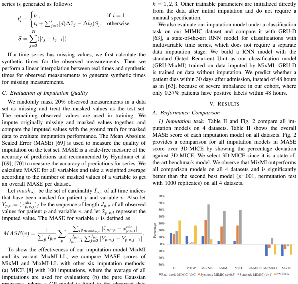
MixMI represents aligned patient data as a patient-by-test-by-time tensor and, for each variable and time index, trains a mixture of three predictive components: a linear regression on the other tests at the same time, a linear regression on the same test at other times, and a per-patient Gaussian process over time. The components are combined not with fixed weights but with individualized mixing weights computed from each patient's observed inputs, which approximate how much responsibility each component should take for that patient. Imputation proceeds iteratively and multiply: several copies of the tensor are filled with random initial guesses, each copy undergoes repeated passes over every variable and time index, and the imputed values are averaged across copies. The paper reports that MixMI outperforms all comparison models on all four datasets and is significantly better than the second-best model, and that the individualized-weight version beats its fixed-weight counterpart by 9.73% in MASE on the synthetic real-world-derived dataset.

Load-bearing premise

The load-bearing premise is that the time tensor is completely known and that, for a given patient, all tests at a time index share the same timestamp; if real laboratory draws occur at different times per analyte, the Gaussian-process component is trained on artificial spacings.

Editorial extensions

If this is right

Every one of the 13 laboratory variables in the real-world cohort is imputed with lower MASE by MixMI or MixMI-LL than by any comparison model, so the advantage is not driven by a single test.
Because MixMI is a pure imputer, any downstream classifier or regressor can be trained on the completed data; the paper demonstrates parity with a no-imputation recurrent model on a 30-day mortality classification task.
The individualized-weight mechanism generalizes beyond Gaussian processes: any mixture component whose predictive confidence varies per input can be weighted this way.
The automatic choice between the linear-only and full Gaussian-process variants makes the method usable without knowing in advance whether temporal structure is strong enough to justify Gaussian processes.
Multiple copies and iterative passes follow the multiple-imputation paradigm, so the spread across copies can serve as a measure of imputation uncertainty.

Reading between the lines

Editorial extensions of the paper, not claims the author makes directly.

A testable extension the paper leaves open is replacing the squared-exponential Gaussian-process kernel with periodic or Matern kernels; longer intensive-care stays often have circadian laboratory rhythms that the current kernel may not capture.
If the shared-timestamp assumption is violated, one could run MixMI on each analyte's actual clock time and treat the change in MASE as a measure of how much of the claimed gain is real temporal signal rather than an artifact of alignment.
The individualized mixing weight could itself be learned as a function of the input, for example through a small neural gating network, instead of being fixed as a posterior ratio; that would let the model adapt across datasets with different missingness mechanisms, though the paper does not test this.
The 30-day mortality experiment ties with a no-imputation recurrent model on AUC, suggesting that the immediate practical payoff may be improved data quality for other tasks rather than a direct classification lift on this particular outcome.

Share X Bluesky LinkedIn Reddit HN

Signed reviews

No signed human review yet.

Editorial analysis

A structured set of objections, weighed in public.

Desk editor's note, referee report, and a circularity audit.

Desk Editor's Note

read the letter

The one thing to know: this is a serious imputation paper with a genuinely new modeling idea, but the headline 'all 4 datasets' significance claim rests partly on synthetic benchmarks that leak the true missing value into the time covariate. The real-world results are still worth taking seriously.

What is actually new: MixMI mixes two linear regressions (cross-sectional and temporal) with a GP, and learns per-patient mixing weights from the data via EM. That individualized weight mechanism is a real step beyond fixed-weight mixtures like MGP or the ad hoc weighting in 3D-MICE. The model equations are coherent, the EM updates in Appendix A are standard and correct, and the authors compare against a reasonable set of baselines (MICE, M-RNN, GMM, GP, MTGP, 3D-MICE) on two real datasets. Code is public. The MIMIC-III results in Table II show a solid improvement over 3D-MICE (0.093 vs 0.112 MASE), and the variable-wise table shows consistent gains. The classification downstream test ties with GRU-D, which is fine for an imputation paper.

The soft spots, in order of severity. First, the synthetic data construction in Section IV.B is contaminated. The synthetic time for an observed measurement depends on Δx, which includes the actual measurement value. Masking is applied after these times are computed, so for every masked test point, the time covariate fed to every model is a function of the true value being predicted. Any smooth temporal model can exploit that. This invalidates the two 'Synthetic MIMIC' rows in Table II and the claim of significance on all 4 datasets at p=.001. I checked the equations; the leak is real. Second, the evaluation uses a single random 20% mask per dataset, so we have no sense of variance across masks. The permutation test only resamples within that one mask. Third, the paper assumes that, for a given patient, all lab tests at a time index share the same timestamp, while raw EHR draws are at different times. The alignment procedure is not described, so the GP component's inputs may be partly artificial on the real datasets.

Who this is for: researchers working on EHR imputation or mixture models for time series. The model idea is worth borrowing, and the real-world results suggest MixMI is competitive. It doesn't open a new area, but it's a useful contribution. With the synthetic leakage fixed and repeated-mask variance reported, this could be a solid paper. I'd send it to referee, but the authors should be asked to address the leak and the timestamp assumption.

Referee Report

3 major / 4 minor

Summary. The paper proposes MixMI, a mixture-based multiple imputation model for multivariable clinical time series. It combines two linear-regression views (cross-sectional and temporal) with a Gaussian-process component and introduces individualized per-patient mixing weights, trained via the EM algorithm. The model is evaluated against six benchmarks on two real EHR datasets (MIMIC-III and NMEDW) and on two synthetic MIMIC variants with different temporal-correlation strengths, using MASE for imputation accuracy and AUC for a downstream mortality-prediction task.

Significance. The model formulation is coherent, the EM updates are standard, and an open-source implementation is provided. If the reported results are sound, MixMI is a useful contribution to clinical time-series imputation, offering a statistically grounded alternative to heuristic weighting schemes such as 3D-MICE. The real-world results suggest the model is competitive, and the study includes a downstream classification comparison with GRU-D. However, the synthetic-data evaluation is contaminated by label leakage, and the significance testing rests on a single random mask, so the paper's headline 'all 4 datasets' claim is not currently supported.

major comments (3)

[IV.B–IV.C] The synthetic time generation in Section IV.B is a function of the true measurement values: t'_i = t_i + sum_{j=2..i} d(Dx_j - Dt_j) S, with Dx_j = |x_j - x_{j-1}| / sum_{k=2..B} |x_k - x_{k-1}|. Since the 20% masking in Section IV.C is applied only after these times are computed, every masked value has its time covariate (and hence the GP input) depending on the value the imputation model is asked to predict. This is a label-leakage flaw that contaminates the two Synthetic MIMIC rows of Table II and invalidates the Section V.A.1 statement that MixMI is significantly better than the second-best model on all 4 datasets. The real-world MIMIC and NMEDW rows are not affected by this flaw, but the synthetic comparison should be redesigned (e.g., compute times from observed values only) and the affected claims re-stated.
[V.A.1] The significance claim relies on a permutation test with 1000 replicates performed within a single random 20% mask. With only one mask, the p=.001 can only describe whether the gap between MixMI and the second-best model is unexpected under permutation of that particular test set; it does not control for variability across masks or across data splits. To support the claim that MixMI is significantly better across datasets, the authors should evaluate on multiple independent masks (e.g., 5–10) and report the distribution of MASE scores and a paired test across masks.
[III.A] The model assumes a complete time tensor T with t_{p,v,b}=t_{p,u,b} for all laboratory tests v,u for a given patient p at time index b. Raw EHR laboratory results are typically drawn at different clock times for different analytes, and the paper does not describe how admissions are aligned into B common time indices or how timestamps are assigned. If the alignment uses arbitrary or approximated timestamps, the GP component's squared-exponential covariance is evaluated on artificial inputs, and the claimed temporal advantage on the real-world datasets is not established. The authors should either justify the equal-timestamp assumption for the cohorts used or provide a sensitivity analysis with per-variable times.

minor comments (4)

[Author affiliations] The first author's affiliation is spelled 'Northwester University' in the header; please correct to 'Northwestern University'.
[V.C] The comparison in Section V.C reports an improvement from 0.08351 to 0.07538 without identifying the dataset or setting; these numbers appear to correspond to the Synthetic MIMIC (d=1) row in Table II, and the text should make that explicit.
[Table II] The footnote 'MTGP cannot have multiple inputs, thus not applicable to the synthetic datasets' is unclear, since MTGP is designed for multi-task settings with multiple outputs; please explain precisely why MTGP is inapplicable to the synthetic benchmark.
[IV.C] In the MASE definition, the scaling term J_{p,v}/(J_{p,v}-1) is nonstandard; please clarify that the denominator is the mean absolute error of the naive one-step-ahead forecast on the observed part of each series, and describe how series with J_p,v = 1 are handled.

Circularity Check

1 steps flagged · score 6.0 of 10

Synthetic MIMIC benchmark leaks the true masked value into the synthetic time covariate, making the 'all 4 datasets' significance claim partly circular by construction.

self definitional [Section IV.B (Synthetic Datasets), equations for ∆x̃ and t′; Section IV.C (Evaluation of Imputation Quality)]
"∆x̃i = |xi−xi−1|∑B i=2|xi−xi−1| ... t′i = { t1, if i = 1; ti + ∑i j=2[d(∆x̃j− ∆t̃j)S], otherwise } ... We randomly mask 20% observed measurements in a data set as missing and treat the masked values as the test set. We impute originally missing and masked values together, and compare the imputed values with the ground truth for masked data to evaluate imputation performance."

The synthetic time covariate fed to every imputation model is computed from ∆x̃j, whose numerator is |xi−xi−1| for the very measurement xi that Section IV.C later masks as a test value. Thus the input time tensor is defined in terms of the ground-truth output being predicted. For the Synthetic MIMIC rows of Table II, a temporal model (MixMI's GP component, or MICE/GMM with time as a feature) is handed information about the masked value's relation to its neighbors, so those predictions are partly forced by construction. The 'all 4 datasets' p=.001 claim in Section V.A.1 relies on these rows; real-world MIMIC and NMEDW rows are unaffected, but the headline claim is partially circular.

full rationale

The mathematical derivation of MixMI is self-contained: the mixture model, EM updates, and individualized weights Π are defined from the observed tensor and fitted parameters, not from the test targets, and no self-citation carries a load-bearing premise (3D-MICE [41] is used only as a benchmark and dataset source). However, the synthetic-data evaluation is self-definitional: Section IV.B constructs t′ from the true values xi of measurements that Section IV.C then masks as test labels, so the synthetic experiments do not provide independent predictive evidence. Because the paper's strongest claim is explicitly 'all 4 datasets' with p=.001, this construction contaminates part of the central empirical claim. The real-world MIMIC and NMEDW results remain independent, so the overall circularity is partial rather than total.

Assumptions & free parameters 1 free parameters · 4 assumptions · 0 invented entities

No new physical entities are introduced. The model's assumptions are about data structure and generative form; the main free parameters are model parameters fitted by EM on training data, with initial mixing weights tuned on a validation set.

free parameters (1)

Initial mixing weights π(1), π(2), π(3) = not reported
Tuned on a validation set (Section IV.C); they initialize the EM mixing weights and affect the final mixture.

assumptions (4)

domain assumption All tests for a patient share the same time point within each time index (tp,v,b = tp,u,b).
Section III.A states this, and the complete time tensor T is assumed known. Real EHR lab tests have per-test timestamps; this alignment is not detailed.
domain assumption The joint distribution of measurements and inputs factorizes as a three-component mixture with p(x|V)p(V) within each component (Eq. 7).
This is the generative modeling assumption underlying MixMI.
ad hoc to paper The GP temporal component uses a stationary squared-exponential kernel R(t,t') = exp(-θ|t-t'|^2) with a single length-scale θ.
Appendix B; a standard but arbitrary kernel choice that may not capture nonstationary clinical trajectories.
domain assumption Iterative imputation converges to a stable solution with a few passes.
Section III.A relies on the Gibbs-sampling analogy; no convergence guarantee is given.

how reviews work

0 comments

Cite this review

Pith. "Pith review of Mixture-based Multiple Imputation Model for Clinical Data with a Temporal Dimension." pith.science (2026). https://pith.science/paper/G4MM2Z53

@misc{pith2026190804209,
  author       = {Pith},
  title        = {Pith review of: Mixture-based Multiple Imputation Model for Clinical Data with a Temporal Dimension},
  year         = {2026},
  howpublished = {\url{https://pith.science/paper/G4MM2Z53}},
  note         = {Machine review of arXiv:1908.04209}
}

read the original abstract

The problem of missing values in multivariable time series is a key challenge in many applications such as clinical data mining. Although many imputation methods show their effectiveness in many applications, few of them are designed to accommodate clinical multivariable time series. In this work, we propose a multiple imputation model that capture both cross-sectional information and temporal correlations. We integrate Gaussian processes with mixture models and introduce individualized mixing weights to handle the variance of predictive confidence of Gaussian process models. The proposed model is compared with several state-of-the-art imputation algorithms on both real-world and synthetic datasets. Experiments show that our best model can provide more accurate imputation than the benchmarks on all of our datasets.

Figures

Figures reproduced from arXiv: 1908.04209 by the authors.

**Figure 2.** Percentage deviation of MASE score against 3D-MICE [PITH_FULL_IMAGE:figures/full_fig_p007_2.png] view at source ↗

**Figure 4.** A comparison between individualized mixing weights [PITH_FULL_IMAGE:figures/full_fig_p008_4.png] view at source ↗

Figures from the paper (1 more)

**Figure 3.** Figure 3: Component weights comparison on real-world MIMIC dataset [PITH_FULL_IMAGE:figures/full_fig_p008_3.png]

Discussion (0). Continue with ORCID to comment.

Reference graph

Works this paper leans on

72 extracted references · 70 canonical work pages

[1]

Computa- tional medicine: Translating models to clinical care,

R. L. Winslow, N. Trayanova, D. Geman, and M. I. Miller, “Computa- tional medicine: Translating models to clinical care,” Science Transla- tional Medicine, vol. 4, no. 158, pp. 158rv11–158rv11, 2012

work page 2012
[2]

Ten things we have to do to achieve precision medicine,

I. S. Kohane, “Ten things we have to do to achieve precision medicine,” Science, vol. 349, no. 6243, pp. 37–38, 2015

work page 2015
[3]

Biases introduced by ﬁltering electronic health records for patients with “complete data

G. M. Weber, W. G. Adams, E. V . Bernstam, J. P. Bickel, K. P. Fox, K. Marsolo, V . A. Raghavan, A. Turchin, X. Zhou, S. N. Murphy et al., “Biases introduced by ﬁltering electronic health records for patients with “complete data”,” Journal of the American Medical Informatics Association, vol. 24, no. 6, pp. 1134–1141, 2017

work page 2017
[4]

Efﬁcacy of the indirect approach for estimating structural equation models with missing data: A comparison of ﬁve methods,

R. L. Brown, “Efﬁcacy of the indirect approach for estimating structural equation models with missing data: A comparison of ﬁve methods,” Structural Equation Modeling: A Multidisciplinary Journal, vol. 1, no. 4, pp. 287–316, 1994

work page 1994
[5]

Longitudinal and multi-group modeling with missing data,

W. Wothke, “Longitudinal and multi-group modeling with missing data,” in Modeling longitudinal and multiplegroup data: Practical issues, applied approaches, and speciﬁc examples, T. D. Little, K. U. Schnabel, and J. Baumert, Eds., 2000, pp. 219–240

work page 2000
[6]

Full information estimation in the presence of in- complete data,

J. L. Arbuckle, “Full information estimation in the presence of in- complete data,” in Advanced Structural Equation Modeling: Issues and Techniques, G. A. Marcoulides and R. E. Schumacker, Eds., 1996, vol. 243, p. 277

work page 1996
[7]

Comparison of imputation methods for missing laboratory data in medicine,

A. K. Waljee, A. Mukherjee, A. G. Singal, Y . Zhang, J. Warren, U. Balis, J. Marrero, J. Zhu, and P. D. Higgins, “Comparison of imputation methods for missing laboratory data in medicine,” BMJ Open , vol. 3, no. 8, p. e002847, 2013

work page 2013
[8]

mice: Multivariate imputation by chained equations in r,

S. Buuren and K. Groothuis-Oudshoorn, “mice: Multivariate imputation by chained equations in r,” Journal of Statistical Software, vol. 45, no. 3, 2011

work page 2011

Show all 72 references

[9]

Missing data analysis: Making it work in the real world,

J. W. Graham, “Missing data analysis: Making it work in the real world,” Annual Review of Psychology , vol. 60, pp. 549–576, 2009

2009
[10]

Missing data: Our view of the state of the art

J. L. Schafer and J. W. Graham, “Missing data: Our view of the state of the art.” Psychological Methods, vol. 7, no. 2, p. 147, 2002

2002
[11]

Multiple imputations in sample surveys-a phenomeno- logical bayesian approach to nonresponse,

D. B. Rubin, “Multiple imputations in sample surveys-a phenomeno- logical bayesian approach to nonresponse,” in Proceedings of the survey research methods section of the American Statistical Association , vol. 1. American Statistical Association, 1978, pp. 20–34

1978
[12]

John Wiley & Sons, 1987

——, Multiple imputation for nonresponse in surveys . John Wiley & Sons, 1987

1987
[13]

J. L. Schafer, Analysis of incomplete multivariate data . Chapman and Hall/CRC, 1997

1997
[14]

A multivariate technique for multiply imputing missing values using a sequence of regression models,

T. E. Raghunathan, J. M. Lepkowski, J. Van Hoewyk, and P. Solenberger, “A multivariate technique for multiply imputing missing values using a sequence of regression models,” Survey Methodology, vol. 27, no. 1, pp. 85–96, 2001

2001
[15]

Van Buuren, Flexible imputation of missing data

S. Van Buuren, Flexible imputation of missing data . Chapman and Hall/CRC, 2018

2018
[16]

Fully conditional speciﬁcation in multivariate imputation,

S. Van Buuren, J. P. Brand, C. G. Groothuis-Oudshoorn, and D. B. Ru- bin, “Fully conditional speciﬁcation in multivariate imputation,” Journal of statistical computation and simulation, vol. 76, no. 12, pp. 1049–1064, 2006

2006
[17]

Multiple imputation for the comparison of two screening tests in two-phase alzheimer studies,

O. Harel and X.-H. Zhou, “Multiple imputation for the comparison of two screening tests in two-phase alzheimer studies,” Statistics in Medicine, vol. 26, no. 11, pp. 2370–2388, 2007

2007
[18]

A comparison of multiple imputation and fully augmented weighted estimators for cox regression with missing covariates,

L. Qi, Y .-F. Wang, and Y . He, “A comparison of multiple imputation and fully augmented weighted estimators for cox regression with missing covariates,”Statistics in Medicine, vol. 29, no. 25, pp. 2592–2604, 2010

2010
[19]

Multiple imputation with diagnostics (mi) in r: Opening windows into the black box,

Y .-S. Su, A. Gelman, J. Hill, M. Yajima et al., “Multiple imputation with diagnostics (mi) in r: Opening windows into the black box,” Journal of Statistical Software, vol. 45, no. 2, pp. 1–31, 2011

2011
[20]

Survival anal- ysis using auxiliary variables via non-parametric multiple imputation,

C.-H. Hsu, J. M. Taylor, S. Murray, and D. Commenges, “Survival anal- ysis using auxiliary variables via non-parametric multiple imputation,” Statistics in Medicine , vol. 25, no. 20, pp. 3503–3517, 2006

2006
[21]

Doubly robust nonparametric multiple imputation for ignorable missing data,

Q. Long, C.-H. Hsu, and Y . Li, “Doubly robust nonparametric multiple imputation for ignorable missing data,” Statistica Sinica, vol. 22, p. 149, 2012

2012
[22]

Multiple imputation of missing blood pressure covariates in survival analysis,

S. Van Buuren, H. C. Boshuizen, and D. L. Knook, “Multiple imputation of missing blood pressure covariates in survival analysis,” Statistics in Medicine, vol. 18, no. 6, pp. 681–694, 1999

1999
[23]

Multiple imputation for general missing data patterns in the presence of high-dimensional data,

Y . Deng, C. Chang, M. S. Ido, and Q. Long, “Multiple imputation for general missing data patterns in the presence of high-dimensional data,” Scientiﬁc Reports, vol. 6, p. 21689, 2016

2016
[24]

Missforest—non-parametric missing value imputation for mixed-type data,

D. J. Stekhoven and P. B ¨uhlmann, “Missforest—non-parametric missing value imputation for mixed-type data,” Bioinformatics, vol. 28, no. 1, pp. 112–118, 2011

2011
[25]

Robust likelihood-based analysis of multivariate data with missing values,

R. Little and H. An, “Robust likelihood-based analysis of multivariate data with missing values,” Statistica Sinica, pp. 949–968, 2004

2004
[26]

Using machine learning to predict laboratory test results,

Y . Luo, P. Szolovits, A. S. Dighe, and J. M. Baron, “Using machine learning to predict laboratory test results,” American Journal of Clinical Pathology, vol. 145, no. 6, pp. 778–788, 2016

2016
[27]

Extensions of the penalized spline of propensity prediction method of imputation,

G. Zhang and R. Little, “Extensions of the penalized spline of propensity prediction method of imputation,” Biometrics, vol. 65, no. 3, pp. 911– 918, 2009

2009
[28]

Missing value estimation methods for dna microarrays,

O. Troyanskaya, M. Cantor, G. Sherlock, P. Brown, T. Hastie, R. Tibshi- rani, D. Botstein, and R. B. Altman, “Missing value estimation methods for dna microarrays,” Bioinformatics, vol. 17, no. 6, pp. 520–525, 2001

2001
[29]

A random-effects model for multiple characteristics with possibly missing data,

A. Shah, N. Laird, and D. Schoenfeld, “A random-effects model for multiple characteristics with possibly missing data,” Journal of the American Statistical Association , vol. 92, no. 438, pp. 775–779, 1997

1997
[30]

Multiple imputation and pos- terior simulation for multivariate missing data in longitudinal studies,

M. Liu, J. M. Taylor, and T. R. Belin, “Multiple imputation and pos- terior simulation for multivariate missing data in longitudinal studies,” Biometrics, vol. 56, no. 4, pp. 1157–1163, 2000

2000
[31]

Computational strategies for multivariate linear mixed-effects models with missing values,

J. L. Schafer and R. M. Yucel, “Computational strategies for multivariate linear mixed-effects models with missing values,” Journal of Computa- tional and Graphical Statistics , vol. 11, no. 2, pp. 437–457, 2002

2002
[32]

Marss: Multivariate autore- gressive state-space models for analyzing time-series data,

E. E. Holmes, E. J. Ward, and K. Wills, “Marss: Multivariate autore- gressive state-space models for analyzing time-series data,” R Journal, vol. 4, no. 1, 2012

2012
[33]

Handling missing data in multivariate time se- ries using a vector autoregressive model-imputation (var-im) algorithm,

F. Bashir and H.-L. Wei, “Handling missing data in multivariate time se- ries using a vector autoregressive model-imputation (var-im) algorithm,” Neurocomputing, 2017

2017
[34]

Learning to detect sepsis with a multitask gaussian process rnn classiﬁer,

J. Futoma, S. Hariharan, and K. Heller, “Learning to detect sepsis with a multitask gaussian process rnn classiﬁer,” in Proceedings of the 34th International Conference on Machine Learning-Volume 70. JMLR. org, 2017, pp. 1174–1182

2017
[35]

Multi-task gaussian process prediction,

E. V . Bonilla, K. M. Chai, and C. Williams, “Multi-task gaussian process prediction,” in Advances in Neural Information Processing Systems , 2008, pp. 153–160

2008
[36]

A functional multiple impu- tation approach to incomplete longitudinal data,

Y . He, R. Yucel, and T. E. Raghunathan, “A functional multiple impu- tation approach to incomplete longitudinal data,” Statistics in Medicine , vol. 30, no. 10, pp. 1137–1156, 2011

2011
[37]

A functional data approach to missing value imputation and outlier detection for trafﬁc ﬂow data,

J.-M. Chiou, Y .-C. Zhang, W.-H. Chen, and C.-W. Chang, “A functional data approach to missing value imputation and outlier detection for trafﬁc ﬂow data,” Transportmetrica B: Transport Dynamics, vol. 2, no. 2, pp. 106–129, 2014

2014
[38]

A bayesian approach to functional mixed-effects modeling for longitudinal data with binomial outcomes,

S. Kliethermes and J. Oleson, “A bayesian approach to functional mixed-effects modeling for longitudinal data with binomial outcomes,” Statistics in Medicine , vol. 33, no. 18, pp. 3130–3146, 2014

2014
[39]

Learning gaussian processes from multiple tasks,

K. Yu, V . Tresp, and A. Schwaighofer, “Learning gaussian processes from multiple tasks,” in Proceedings of the 22nd International Confer- ence on Machine Learning . ACM, 2005, pp. 1012–1019

2005
[40]

Multi-task gaussian process for imputing missing data in multi-trait and multi-environment trials,

T. Hori, D. Montcho, C. Agbangla, K. Ebana, K. Futakuchi, and H. Iwata, “Multi-task gaussian process for imputing missing data in multi-trait and multi-environment trials,” Theoretical and Applied Ge- netics, vol. 129, no. 11, pp. 2101–2115, 2016

2016
[41]

3d-mice: inte- gration of cross-sectional and longitudinal imputation for multi-analyte longitudinal clinical data,

Y . Luo, P. Szolovits, A. S. Dighe, and J. M. Baron, “3d-mice: inte- gration of cross-sectional and longitudinal imputation for multi-analyte longitudinal clinical data,” Journal of the American Medical Informatics Association, vol. 25, no. 6, pp. 645–653, 2017

2017
[42]

Mixtures of gaussian processes,

V . Tresp, “Mixtures of gaussian processes,” in Advances in neural information processing systems , 2001, pp. 654–660

2001
[43]

Imputation through ﬁnite gaussian mixture models,

M. Di Zio, U. Guarnera, and O. Luzi, “Imputation through ﬁnite gaussian mixture models,” Computational Statistics & Data Analysis , vol. 51, no. 11, pp. 5305–5316, 2007

2007
[44]

Efﬁcient em training of gaussian mixtures with missing data,

O. Delalleau, A. Courville, and Y . Bengio, “Efﬁcient em training of gaussian mixtures with missing data,” arXiv preprint arXiv:1209.0521 , 2012

2012 arXiv
[45]

Missing value imputation based on gaussian mixture model for the internet of things,

X. Yan, W. Xiong, L. Hu, F. Wang, and K. Zhao, “Missing value imputation based on gaussian mixture model for the internet of things,” Mathematical Problems in Engineering , vol. 2015, 2015

2015
[46]

Multivariate data imputation using gaussian mixture models,

D. S. Silva and C. V . Deutsch, “Multivariate data imputation using gaussian mixture models,” Spatial statistics, vol. 27, pp. 74–90, 2018

2018
[47]

Tucker factorization with missing data with application to low-n-rank tensor completion,

M. Filipovi ´c and A. Juki ´c, “Tucker factorization with missing data with application to low-n-rank tensor completion,” Multidimensional Systems and Signal Processing , vol. 26, no. 3, pp. 677–692, 2015

2015
[48]

Trace norm regularized candecomp/parafac decomposition with missing data,

Y . Liu, F. Shang, L. Jiao, J. Cheng, and H. Cheng, “Trace norm regularized candecomp/parafac decomposition with missing data,” IEEE Transactions on Cybernetics , vol. 45, no. 11, pp. 2437–2448, 2015

2015
[49]

Tomioka, K

R. Tomioka, K. Hayashi, and H. Kashima. (2010) Estimation of low-rank tensors via convex optimization. [Online]. Available: https://arxiv.org/pdf/1010.0789.pdf

2010 arXiv
[50]

Fast multivariate spatio- temporal analysis via low rank tensor learning,

M. T. Bahadori, Q. R. Yu, and Y . Liu, “Fast multivariate spatio- temporal analysis via low rank tensor learning,” in Advances in Neural Information Processing Systems , 2014, pp. 3491–3499

2014
[51]

Accelerated online low-rank tensor learning for multivariate spatio-temporal streams,

R. Yu, D. Cheng, and Y . Liu, “Accelerated online low-rank tensor learning for multivariate spatio-temporal streams,” in Proceedings of the 32nd International Conference on Machine Learning (ICML-15) , 2015, pp. 238–247

2015
[52]

Uncovering the spatio-temporal dynamics of memes in the presence of incomplete in- formation,

H. Ge, J. Caverlee, N. Zhang, and A. Squicciarini, “Uncovering the spatio-temporal dynamics of memes in the presence of incomplete in- formation,” inProceedings of the 25th ACM International on Conference on Information and Knowledge Management . ACM, 2016, pp. 1493– 1502

2016
[53]

Autoregressive tensor factor- ization for spatio-temporal predictions,

K. Takeuchi, H. Kashima, and N. Ueda, “Autoregressive tensor factor- ization for spatio-temporal predictions,” IEEE International Conference on Data Mining , 2017

2017
[54]

Facets: Fast comprehensive mining of coevolving high-order time series,

Y . Cai, H. Tong, W. Fan, P. Ji, and Q. He, “Facets: Fast comprehensive mining of coevolving high-order time series,” in Proceedings of the 21th ACM SIGKDD International Conference on Knowledge Discovery and Data Mining. ACM, 2015, pp. 79–88

2015
[55]

Time-aware subgroup matrix decom- position: Imputing missing data using forecasting events,

X. Yang, Y . Zhang, and M. Chi, “Time-aware subgroup matrix decom- position: Imputing missing data using forecasting events,” in 2018 IEEE International Conference on Big Data . IEEE, 2018, pp. 1524–1533

2018
[56]

Stochastic nonparametric event-tensor decomposi- tion,

S. Zhe and Y . Du, “Stochastic nonparametric event-tensor decomposi- tion,” in Advances in Neural Information Processing Systems , 2018, pp. 6855–6865

2018
[57]

Recurrent neural networks for missing or asynchronous data,

Y . Bengio and F. Gingras, “Recurrent neural networks for missing or asynchronous data,” in Advances in neural information processing systems, 1996, pp. 395–401

1996
[58]

A solution for missing data in recurrent neural networks with an application to blood glucose prediction,

V . Tresp and T. Briegel, “A solution for missing data in recurrent neural networks with an application to blood glucose prediction,” in Advances in Neural Information Processing Systems , 1998, pp. 971–977

1998
[59]

Speech recognition with missing data using recurrent neural nets,

S. Parveen and P. Green, “Speech recognition with missing data using recurrent neural nets,” in Advances in Neural Information Processing Systems, 2002, pp. 1189–1195

2002
[60]

Estimating missing data in temporal data streams using multi-directional recurrent neural networks,

J. Yoon, W. R. Zame, and M. van der Schaar, “Estimating missing data in temporal data streams using multi-directional recurrent neural networks,” IEEE Transactions on Biomedical Engineering, vol. 66, no. 5, pp. 1477– 1490, 2018

2018
[61]

Doctor ai: Predicting clinical events via recurrent neural networks,

E. Choi, M. T. Bahadori, A. Schuetz, W. F. Stewart, and J. Sun, “Doctor ai: Predicting clinical events via recurrent neural networks,” in Machine Learning for Healthcare Conference , 2016, pp. 301–318

2016
[62]

Directly modeling missing data in sequences with rnns: Improved classiﬁcation of clinical time series,

Z. C. Lipton, D. Kale, and R. Wetzel, “Directly modeling missing data in sequences with rnns: Improved classiﬁcation of clinical time series,” in Machine Learning for Healthcare Conference , 2016, pp. 253–270

2016
[63]

Recurrent neural networks for multivariate time series with missing values,

Z. Che, S. Purushotham, K. Cho, D. Sontag, and Y . Liu, “Recurrent neural networks for multivariate time series with missing values,” Scientiﬁc reports, vol. 8, no. 1, p. 6085, 2018

2018
[64]

Predicting icu readmission using grouped physiological and medication trends,

Y . Xue, D. Klabjan, and Y . Luo, “Predicting icu readmission using grouped physiological and medication trends,” Artiﬁcial Intelligence in Medicine, 2018

2018
[65]

Parameterization and bayesian modeling,

A. Gelman, “Parameterization and bayesian modeling,” Journal of the American Statistical Association , vol. 99, no. 466, pp. 537–545, 2004

2004
[66]

Mimic-iii, a freely accessible critical care database,

A. E. Johnson, T. J. Pollard, L. Shen, H. L. Li-wei, M. Feng, M. Ghas- semi, B. Moody, P. Szolovits, L. A. Celi, and R. G. Mark, “Mimic-iii, a freely accessible critical care database,” Scientiﬁc Data , vol. 3, p. 160035, 2016

2016
[67]

A new simpliﬁed acute physiology score (saps ii) based on a european/north american multi- center study,

J.-R. Le Gall, S. Lemeshow, and F. Saulnier, “A new simpliﬁed acute physiology score (saps ii) based on a european/north american multi- center study,” Jama, vol. 270, no. 24, pp. 2957–2963, 1993

1993
[68]

Missing-data adjustments in large surveys,

R. J. Little, “Missing-data adjustments in large surveys,” Journal of Business & Economic Statistics , vol. 6, no. 3, pp. 287–296, 1988

1988
[69]

Another look at measures of forecast accuracy,

R. J. Hyndman and A. B. Koehler, “Another look at measures of forecast accuracy,”International Journal of Forecasting, vol. 22, no. 4, pp. 679– 688, 2006

2006
[70]

A note on the mean absolute scaled error,

P. H. Franses, “A note on the mean absolute scaled error,” International Journal of Forecasting, vol. 32, no. 1, pp. 20–22, 2016

2016
[71]

Gpﬁt: An r package for ﬁtting a gaussian process model to deterministic simulator outputs,

B. MacDonald, P. Ranjan, and H. Chipman, “Gpﬁt: An r package for ﬁtting a gaussian process model to deterministic simulator outputs,” Journal of Statistical Software , vol. 64, no. 1, pp. 1–23, 2015

2015
[72]

K. P. Murphy, Machine learning: a probabilistic perspective . MIT press, 2012. APPENDIX A PARAMETER ESTIMATION IN EM In the E (Expectation) step, we calculate the responsibilities w(k) p,v,b = Qp(qv,b = k) for p∈ Ptr v,b using the current values of the parameters in iteration ...

1989

Pith tools

Reviewed August 14, 2026 · model on record in the stance chip above.

[1] [1]

Computa- tional medicine: Translating models to clinical care,

R. L. Winslow, N. Trayanova, D. Geman, and M. I. Miller, “Computa- tional medicine: Translating models to clinical care,” Science Transla- tional Medicine, vol. 4, no. 158, pp. 158rv11–158rv11, 2012

work page 2012

[2] [2]

Ten things we have to do to achieve precision medicine,

I. S. Kohane, “Ten things we have to do to achieve precision medicine,” Science, vol. 349, no. 6243, pp. 37–38, 2015

work page 2015

[3] [3]

Biases introduced by ﬁltering electronic health records for patients with “complete data

G. M. Weber, W. G. Adams, E. V . Bernstam, J. P. Bickel, K. P. Fox, K. Marsolo, V . A. Raghavan, A. Turchin, X. Zhou, S. N. Murphy et al., “Biases introduced by ﬁltering electronic health records for patients with “complete data”,” Journal of the American Medical Informatics Association, vol. 24, no. 6, pp. 1134–1141, 2017

work page 2017

[4] [4]

Efﬁcacy of the indirect approach for estimating structural equation models with missing data: A comparison of ﬁve methods,

R. L. Brown, “Efﬁcacy of the indirect approach for estimating structural equation models with missing data: A comparison of ﬁve methods,” Structural Equation Modeling: A Multidisciplinary Journal, vol. 1, no. 4, pp. 287–316, 1994

work page 1994

[5] [5]

Longitudinal and multi-group modeling with missing data,

W. Wothke, “Longitudinal and multi-group modeling with missing data,” in Modeling longitudinal and multiplegroup data: Practical issues, applied approaches, and speciﬁc examples, T. D. Little, K. U. Schnabel, and J. Baumert, Eds., 2000, pp. 219–240

work page 2000

[6] [6]

Full information estimation in the presence of in- complete data,

J. L. Arbuckle, “Full information estimation in the presence of in- complete data,” in Advanced Structural Equation Modeling: Issues and Techniques, G. A. Marcoulides and R. E. Schumacker, Eds., 1996, vol. 243, p. 277

work page 1996

[7] [7]

Comparison of imputation methods for missing laboratory data in medicine,

A. K. Waljee, A. Mukherjee, A. G. Singal, Y . Zhang, J. Warren, U. Balis, J. Marrero, J. Zhu, and P. D. Higgins, “Comparison of imputation methods for missing laboratory data in medicine,” BMJ Open , vol. 3, no. 8, p. e002847, 2013

work page 2013

[8] [8]

mice: Multivariate imputation by chained equations in r,

S. Buuren and K. Groothuis-Oudshoorn, “mice: Multivariate imputation by chained equations in r,” Journal of Statistical Software, vol. 45, no. 3, 2011

work page 2011