Simulating Quantum Algorithms Using Fidelity and Coherence Time as Principle Models for Error

Avery Torrance; Daniel Koch; David Kinghorn; Laura Wessing; Paul M. Alsing; Saahil Patel

REVIEW 3 major objections 5 minor 31 references

Simulating Quantum Algorithms Using Fidelity and Coherence Time as Principle Models for Error

T0 review · 3 major / 5 minor · reviewed 2026-08-14 · deepseek-v4-flash

Challenge this review Re-run · record.json Download PDF Read on arXiv ↗ Review JSON

Pith's one-line read Under the paper's two error models, small quantum circuits reach 90% average success only with gate fidelities between 0.99 and 0.999, and Grover iterations need fidelity above 0.9999 or coherence times of about a millisecond.

desk verdict A useful benchmark study of noisy circuits whose coherent-error half is clean but whose decoherence half uses a nonstandard collapse model, so the reported T1 thresholds should be read as specific to that model. read the letter →

arxiv 1908.04229 v2 pith:Z27BEEKJ submitted 2019-08-12 quant-ph

Daniel Koch , Avery Torrance , David Kinghorn , Saahil Patel , Laura Wessing , Paul M. Alsing This is my paper · ORCID

classification quant-ph

keywords quantumalgorithmsgatefidelitycoherencetimeenergyrelaxationerrormodelGrover'salgorithmFouriertransformNISQ

verification ladder T0 review T1 audit T2 compute T3 formal

The pith

A machine-rendered reading of the paper's core claim, the machinery that carries it, and where it could break.

The reading

This paper simulates how two hardware benchmarks—average gate fidelity and coherence time—determine whether small quantum algorithms succeed. The authors build hardware-like circuits for the Bernstein–Vazirani hidden-bit algorithm, the quantum Fourier transform, a controlled-controlled-NOT (CCNOT) gate, and Grover search on a fixed qubit geometry, then inject two single-parameter error models: coherent amplitude errors controlled by $\langle f \rangle$, and energy-relaxation/partial-collapse errors controlled by $T_1$. They report that circuits of roughly 20–30 gates exceed 90% average success once average fidelity lies between 0.99 and 0.999, or once $T_1$ is in the tens to hundreds of microseconds; the deeper Grover circuit needs fidelity above 0.9999 or coherence times near a millisecond. When both error types act together, decoherence is the dominant limit, and the simulated thresholds sit at the edge of what current NISQ hardware promises.

What carries the argument

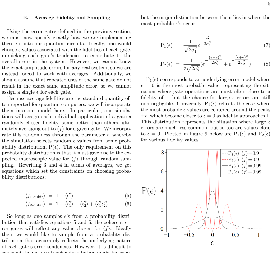
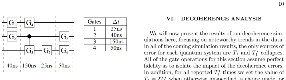
The carrying mechanism is a pair of single-parameter error models plus a discretized time structure. Each coherent error gate is built from a unitary amplitude error: the average gate fidelity is $f = 1 - \epsilon^2$ for one-qubit gates and $f = (1 - \epsilon_1^2)(1 - \epsilon_2^2)$ for two-qubit gates, with $\epsilon$ drawn from one of two zero-mean Gaussian-based distributions whose width is fixed by $\langle f \rangle$. Decoherence is governed by the exponential survival probability $P(\Delta t) = e^{-\Delta t / T_j}$, where $T_j$ is $T_1$ for energy relaxation to $|0\rangle$ and $T_1^* = T_1/2$ for a partial-measurement collapse that renormalizes the superposition. Circuit time is divided into moments, each moment lasting as long as its slowest parallel gate, and after every moment each qubit is randomly collapsed according to $P(\Delta t)$; the identity $\prod_i e^{-\Delta t_i / T_j} = e^{-\sum_i \Delta t_i / T_j}$ makes sequential moment sampling equivalent to one total-time decay. These ingredients convert the two benchmark numbers into predicted success probabilities for each circuit, which is what the paper's thresholds are.

What would settle it

Take one of the simulated circuits, such as one-iteration Grover or QFT, run it on a real device whose per-gate average fidelity and $T_1$ are independently characterized using the same connectivity, and compare the measured average success and run-to-run spread with the paper's curves; if the measurements fall outside the simulation's statistical spread, or if changing only the grouping of gates into parallel moments changes success more than the model predicts, the discrete-moment collapse assumption fails.

Watch

Extended reading notes

Core claim

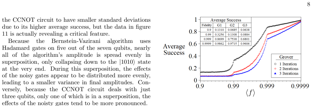
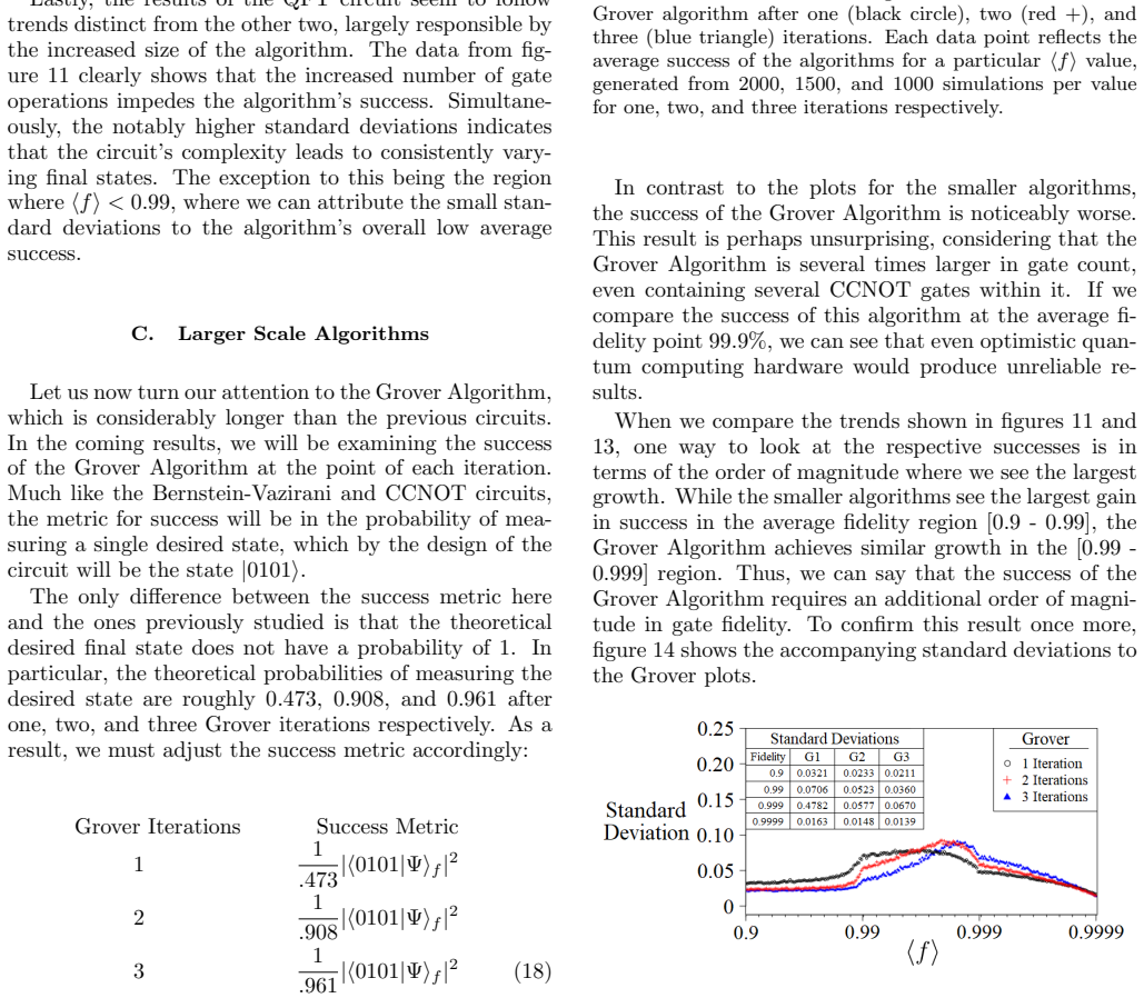
The paper claims that, for these circuits, the average success probability is controlled almost entirely by the aggregate quality numbers $\langle f \rangle$ and $T_1$, with partial-measurement collapse time set to $T_1^* = T_1/2$. Under gate fidelity errors alone, the smaller Bernstein–Vazirani, CCNOT, and QFT circuits achieve greater than 90% average success for average fidelities in the range 0.99–0.999, while one to three Grover iterations require fidelities upward of 0.9999. Under decoherence errors alone, the same 90% threshold needs coherence times of order 50–500 µs: about 30 µs for the shortest circuit, 61 µs for QFT, and 425–975 µs for one to three Grover iterations. With both error models combined, the small circuits cross 90% only near $\langle f \rangle \approx 0.997$ and $T_1 \approx 80$ µs, and the authors conclude that improving coherence time, not fidelity, yields the largest near-term gains. They also find that the detailed shape of the underlying error distribution matters little, and that a single decoherence collapse, especially the first, accounts for most of the damage.

Load-bearing premise

The reported thresholds rest on the modeling premise that decoherence happens only as instantaneous collapses at discrete moments between parallel gate groups, and that the partial-measurement time $T_1^*$ is exactly half of $T_1$; if real qubits decohere continuously during gates, or if that half-times relation is wrong, the 50–500 µs numbers shift substantially.

Editorial extensions

If this is right

Smaller circuits—Bernstein–Vazirani, CCNOT, and QFT—exceed 90% average success with gate fidelities between 0.99 and 0.999 when gate error is the only noise source.
The same small circuits reach 90% average success under decoherence alone with coherence times near 30–60 µs, while one to three Grover iterations need 425–975 µs.
With both error sources active, the small circuits cross 90% only near $\langle f \rangle \approx 0.997$ and $T_1 \approx 80$ µs, and coherence time, not gate fidelity, is the limiting resource.
Grover circuits of the depth studied are beyond current NISQ devices: they need gate fidelity above 0.9999 or near-millisecond $T_1$.
The first decoherence collapse causes the largest drop in average success; subsequent collapses have smaller additional impact, so preventing early collapses matters most.

Reading between the lines

Editorial extensions of the paper, not claims the author makes directly.

Because the simulations omit dephasing ($T_2$), which the paper lists as future work, the reported $T_1$ thresholds are likely optimistic for full device noise; adding $T_2$ should push the required coherence times and fidelities upward.
The moment-based timing model implies that circuit scheduling is itself a noise parameter: recompiling the same algorithm to balance parallel moments and shorten each moment's longest gate should reduce decoherence without changing the gate count, a testable extension the paper does not run.
The observed favorable single-collapse boosts in Grover suggest a possible error-mitigation strategy for algorithms whose ideal final state has probability below 1: deliberately steering a partial collapse toward the desired outcome. This is an extension, not something the paper proposes.
The insensitivity to the error distribution $P_1(\epsilon)$ versus $P_2(\epsilon)$ assumes zero-mean errors; real devices with biased errors could make average fidelity alone an incomplete benchmark, and bias-aware metrics would need testing.

Share X Bluesky LinkedIn Reddit HN

Signed reviews

No signed human review yet.

Editorial analysis

A structured set of objections, weighed in public.

Desk editor's note, referee report, and a circularity audit.

Desk Editor's Note

read the letter

Daniel, here's the short version. This is a legitimate forward simulation of Bernstein-Vazirani, QFT, and Grover on a ladder connectivity graph, with noisy gates and decoherence. What's actually new is the specific combination: the coherent amplitude error model with Gaussian-sampled epsilon, the connectivity-restricted circuits, and the breakpoint numbers—roughly 0.99–0.999 average fidelity for small circuits, above 0.9999 for Grover, and T1 around 50–500 µs for decoherence-only. The math of the coherent error model checks out: equations 13–16 enforce the average fidelity constraints, and f=1-epsilon^2 is consistent with a unitary implementation. The authors also test two epsilon distributions and show the average-success results don't depend on which one you use, which is a good robustness check.

The soft spots are real but mostly addressable. The decoherence model is not standard. They let T1 collapse only qubits already in |1>, and for superpositions they use a T*1 partial-measurement channel with probability decay, then set T*1 = T1/2. Physical amplitude damping acts on the |1> amplitude of a superposition continuously and doesn't require the qubit to be classical |1>; and the T*1 = T1/2 relation isn't the usual 1/T2 = 1/(2T1) + 1/T_phi. So the headline T1 thresholds are sensitive to a modeling choice rather than a direct description of open-system dynamics. The paper acknowledges missing T2 and per-qubit variation as future work, but the abstract and conclusion don't carry that caveat. That's a load-bearing weakness for the coherence-time claims, though not for the fidelity thresholds.

Also minor: gate times in figure 16 are uncited representative values, and no code or data accompanies the paper, so the numbers are hard to reproduce exactly. And calling 90% average success 'reliably successful' is too strong given the large standard deviations shown in their own figures.

Bottom line: the fidelity-side results are worth taking seriously, and the study is a reasonable order-of-magnitude benchmark. The T1 numbers should not be quoted without the model caveat. The paper deserves a serious referee; I'd send it out, with requests for code/data and a sensitivity analysis on the T1/T*1 ratio and gate times. I wouldn't cite the coherence thresholds as physical, but the circuit-construction and fidelity-model portions are solid enough for a reading-group discussion.

Referee Report

3 major / 5 minor

Summary. The paper proposes a connectivity-limited qubit geometry, constructs adapted circuits for the Bernstein-Vazirani, QFT, and Grover algorithms on that geometry, and simulates them under two error models: a coherent amplitude-error model parameterized by average gate fidelity, and a decoherence model combining T1 energy relaxation with a partial-collapse process T1*. The simulations report average success rates and derive benchmark thresholds for gate fidelity and coherence time needed for high-probability success. The central quantitative claims are that smaller algorithms require average fidelities around 0.99-0.999 and T1 of order 50-500 microseconds, while Grover iterations require fidelities above 0.9999 and longer coherence times. The paper concludes that circuit depth and gate count dominate the success rates and that decoherence errors are the main limiting factor.

Significance. If the reported thresholds were robust, they would give useful NISQ-era hardware targets. The paper has several genuine strengths: the simulation methodology is a forward state-vector evolution rather than a fit to the success metric; the fidelity constraints in Eqs. (5)-(6) and (13)-(16) are internally consistent; and the comparison of two zero-mean error distributions is a reasonable first test of model sensitivity. The paper also makes a concrete attempt to include realistic connectivity constraints. However, the significance is substantially weakened by the nonstandard decoherence model and by representative, uncited gate times, so the quantitative thresholds are not directly comparable to standard T1/T2 hardware specifications. The qualitative conclusions about circuit depth and error accumulation are credible, but the headline numbers require either a reformulation using standard amplitude-damping/dephasing channels or a clear limitation statement.

major comments (3)

[V.A and Eqs. (20)-(22)] The decoherence model is nonstandard: T1 is applied only to qubits that are in the |1> computational basis state, while superpositions are subjected to T1* as a projective partial measurement onto |0> or |1>. Physical T1 amplitude damping acts continuously on the |1> amplitude of any superposition, and physical dephasing does not project onto basis states. The paper sets T1* = T1/2 (Section VI) without a physical justification and acknowledges in Section VIII that T2 is missing. Because Fig. 22 shows the combined-error thresholds tracking the decoherence-only curves more than the fidelity-only curves, the reported required coherence times (Section VIII) are an artifact of this modeling choice. This issue is load-bearing for the central claim and needs to be addressed either by rerunning with standard amplitude-damping and dephasing channels or by explicitly restricting the claims to this specific collapse model and justifying its physical relevance.
[V.A and Fig. 16] The gate times used to compute circuit times are described as 'based on average results found from reports for 1 and 2-qubit gates on superconducting qubits,' but no references are given. The T1 thresholds scale directly with the total circuit time through Eq. (19), so changing these representative times shifts the reported 50-500 microsecond range. Without citations or a sensitivity analysis over plausible gate times, the quantitative coherence-time thresholds are not robust. A revision should provide sources for these values or demonstrate how the conclusions change when they are varied.
[VIII and Abstract] The conclusion states that the required fidelities 'ranged from 0.99≥⟨f⟩≥0.999' and the required coherence times 'were of the order 50µs≥T1≥500µs.' The inequality directions are reversed: these should presumably read 0.99≤⟨f⟩≤0.999 and 50µs≤T1≤500µs. More importantly, the T1 range contradicts Fig. 18, where the Grover iterations reach 90% success only at T1 = 425µs, 745µs, and 975µs. As written, the central summary misstates the paper's own results and should be corrected.

minor comments (5)

[III.A] The phrase 'isolated isolate each source of error' contains a typo and should read 'isolate each source of error.'
[IV.B] The text says 'the eﬀects of the noisty gates' — 'noisty' should be 'noisy.'
[VI] The relation T1 = 2T1* is introduced 'for simplicity reasons' but not connected to the standard relation 1/T2 = 1/(2T1) + 1/Tφ; if T1* is meant to capture dephasing-like processes, this connection should be clarified.
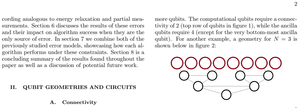
[II.A] The notation '2N computational qubits' is ambiguous; it should be clear whether this means 2^N or 2N, and the example N=2 suggests the latter but could be stated explicitly.
[IV.A] The conclusion that the choice of P(ε) has no impact is based on two zero-mean Gaussian distributions; the paper correctly notes that biased distributions could change this, but the statement 'any probability distribution that satisfies ⟨ϵ⟩=0 will lead to the same average success' is stronger than the evidence supports.

Circularity Check

0 steps flagged · score 0.0 of 10

No significant circularity: the reported fidelity and coherence-time thresholds are forward-simulation outputs, not fitted or redefined inputs.

full rationale

The paper's central claims—the fidelity and T1 values needed to reach high average success—are obtained by sweeping input parameters and computing success probabilities from the simulated final state amplitudes. The coherent-error model constrains the sampled epsilon distribution to reproduce an input average fidelity <f>, but that constraint is an input to the simulation, not a fit to the success metric. Likewise, the decoherence model applies T1 and T*1 collapse events with probabilities from exp(-Δt/Tj); the reported 50–500 µs T1 thresholds are outputs of those simulations. The choice T*1 = T1/2 is a stated modeling assumption whose physical realism may be questioned, but that is a correctness or model-risk concern, not circularity. The sole self-citation (ref. [22]) appears in a general remark about noise impact and is not load-bearing for the derivation. No prediction in the paper reduces by construction to an input parameter, and no uniqueness theorem or ansatz is imported from prior work to force the conclusions. The paper is not benchmarked against external devices, but absence of external validation is not circularity.

Assumptions & free parameters 6 free parameters · 6 assumptions · 1 invented entities

The paper's results are forward simulations; the outputs are not fitted to data. However, several load-bearing inputs are chosen by the authors (gate times, T1* ratio, start point and improvement rates for the combined model, circuit parallelization). The coherent error model and the T1* collapse process are phenomenological inventions rather than measurements.

free parameters (6)

1-qubit gate time = not given numerically, see figure 16
Used to set moment lengths and therefore T1/T1* collapse probabilities; chosen as representative values without a cited source.
2-qubit gate time = not given numerically, see figure 16
Approximately five times longer than 1-qubit gates; heavily influences total circuit time and decoherence exposure.
T1* / T1 ratio = 0.5
Set for simplicity in all decoherence simulations; changing this ratio changes the partial-collapse probability and thus the success curves.
Initial combined-model fidelity and T1 = 0.99 and 20 us
Starting point for figure 22; different starting values would shift the combined-success curves along the x-axis.
Combined-model improvement rates = 10% fidelity, 5% T1 per step
Chosen as plausible technological improvement rates; they set the spacing of points in figure 22.
Circuit parallelization choices = BV CNOTs serial; Grover CCNOTs partially parallel
Affects circuit depth; the paper states that CNOT parallelization is possible but not used for BV, and some Grover CCNOTs are parallelized.

assumptions (6)

domain assumption A gate error can be modeled by a unitary matrix whose fidelity with the ideal gate is controlled by a single amplitude parameter (equations 2-4 and figure 8).
The paper invents this coherent amplitude error model; it is not derived from a physical noise process.
domain assumption Errors on the control and target qubits of a 2-qubit gate are independent and share the same average fidelity (equation 12 and the text after equation 16).
Real crosstalk can induce correlated errors; the paper assumes independence without justification.
ad hoc to paper Decoherence collapses are applied only at circuit moments, with the time step set by the longest gate in the moment, and no decoherence occurs during gate execution (section V.A, figure 15).
This discretization is a modeling choice made for simulation simplicity; continuous decoherence could change the quantitative results.
ad hoc to paper Energy relaxation T1 applies only to qubits in the pure |1> state, while partial collapses of superposition states are governed by a separate parameter T1* (equations 20-22).
This split is invented for the paper; standard amplitude-damping models treat T1 continuously for any state.
domain assumption The ladder geometry with four nearest-neighbor connections is realistic and the circuits in figures 3-6 are the exact instructions used in the simulation (section II).
The paper asserts the geometry maps to existing chips, and some circuit details differ from the diagrams (e.g., parallelized Grover CCNOTs).
standard math Standard quantum mechanics and the circuit model hold.
Background assumption needed for any simulation.

invented entities (1)

T1* partial collapse parameter
purpose: A phenomenological rate for spontaneous partial-measurement collapses during superposition, with probability exp(-Delta t / T1*)
No independent evidence that such a process exists as modeled; the paper sets T1* = T1/2 arbitrarily and does not connect it to a physical mechanism.

how reviews work

0 comments

Cite this review

Pith. "Pith review of Simulating Quantum Algorithms Using Fidelity and Coherence Time as Principle Models for Error." pith.science (2026). https://pith.science/paper/Z27BEEKJ

@misc{pith2026190804229,
  author       = {Pith},
  title        = {Pith review of: Simulating Quantum Algorithms Using Fidelity and Coherence Time as Principle Models for Error},
  year         = {2026},
  howpublished = {\url{https://pith.science/paper/Z27BEEKJ}},
  note         = {Machine review of arXiv:1908.04229}
}

read the original abstract

As various quantum computing technologies continue to compete for quantum supremacy, several parameters have emerged as benchmarks for the quality of qubits. These include fidelity, coherence times, connectivity, and a few others. In this paper, we aim to study the importance of these parameters and their impact on quantum algorithms. We propose a realistic connectivity geometry and form quantum circuits for the Bernstein-Vazirani, QFT, and Grover Algorithms based on the limitations of the chosen geometry. We then simulate these algorithms using error models to study the impact of gate fidelity and coherence times on success of the algorithms. We report on the findings of our simulations and note the various benchmarking values which produce reliably successful results.

Figures

Figures reproduced from arXiv: 1908.04229 by the authors.

**Figure 1.** FIG. 1: Top row of qubits marked by “Q” (dark red): compu [PITH_FULL_IMAGE:figures/full_fig_p002_1.png] view at source ↗

**Figure 5.** FIG. 5: Decomposition of the CCNOT gate into 1 and 2-qubit [PITH_FULL_IMAGE:figures/full_fig_p003_5.png] view at source ↗

Figures from the paper (18 more)

**Figure 3.** Figure 3: FIG. 3: Quantum circuit for the Bernstein-Vazirani Algo [PITH_FULL_IMAGE:figures/full_fig_p003_3.png]

**Figure 6.** Figure 6: FIG. 6: Quantum Circuit for the Grover Algorithm. The [PITH_FULL_IMAGE:figures/full_fig_p003_6.png]

**Figure 8.** Figure 8: FIG. 8: Matrix representations of each 1 and 2-qubit gate [PITH_FULL_IMAGE:figures/full_fig_p004_8.png]

**Figure 7.** Figure 7: shows an example of a coherent amplitude error, whereby the X˜ transformation results in a final state that is displaced from the ideal final state by an angle of sin−1 (). Using the definition of fidelity from equation 1 in conjunction with U˜ from equation 2, we…

**Figure 9.** Figure 9: FIG. 9: Plots for P [PITH_FULL_IMAGE:figures/full_fig_p005_9.png]

**Figure 10.** Figure 10: FIG. 10: (top) Average success of the Bernstein-Vazirani Al [PITH_FULL_IMAGE:figures/full_fig_p006_10.png]

**Figure 11.** Figure 11: figure 11. While the Bernstein-Vazirani algorithm is per [PITH_FULL_IMAGE:figures/full_fig_p006_11.png]

**Figure 11.** Figure 11: FIG. 11: Plotted are the average values of success for the [PITH_FULL_IMAGE:figures/full_fig_p007_11.png]

**Figure 12.** Figure 12: FIG. 12: Plotted are the standard deviations for the CCNOT [PITH_FULL_IMAGE:figures/full_fig_p007_12.png]

**Figure 13.** Figure 13: FIG. 13: Plotted are the average values of success for the [PITH_FULL_IMAGE:figures/full_fig_p008_13.png]

**Figure 14.** Figure 14: FIG. 14: Plotted are the standard deviations for the three [PITH_FULL_IMAGE:figures/full_fig_p008_14.png]

**Figure 15.** Figure 15: FIG. 15: Example circuit showing the resulting times for each [PITH_FULL_IMAGE:figures/full_fig_p010_15.png]

**Figure 17.** Figure 17: FIG. 17: The average success rates of the Bernstein-Vazirani [PITH_FULL_IMAGE:figures/full_fig_p010_17.png]

**Figure 19.** Figure 19: FIG. 19: The sum of the total amount of time in each cir [PITH_FULL_IMAGE:figures/full_fig_p011_19.png]

**Figure 18.** Figure 18: FIG. 18: The average success of the Grover Algorithm at [PITH_FULL_IMAGE:figures/full_fig_p011_18.png]

**Figure 20.** Figure 20: FIG. 20: Success rates for the Grover Algorithm (1 Iteration) [PITH_FULL_IMAGE:figures/full_fig_p012_20.png]

**Figure 21.** Figure 21: FIG. 21: Plotted are the average success rates for the [PITH_FULL_IMAGE:figures/full_fig_p012_21.png]

**Figure 22.** Figure 22: FIG. 22: Average success rate as a function of both sources of [PITH_FULL_IMAGE:figures/full_fig_p013_22.png]

Discussion (0). Continue with ORCID to comment.

Reference graph

Works this paper leans on

31 extracted references · 23 canonical work pages

[1]

IBM Quantum Experience, quantum- computing.ibm.com. (2019)

work page 2019
[2]

mo- ments

(4) 5 B. Average Fidelity and Sampling Using the error gates deﬁned in the previous section, we must now specify exactly how we are implementing these ϵ’s into our quantum circuits. Ideally, one would chooseϵ values associated with the ﬁdelities of each gate, mimicking each gate’s tendencies to contribute to the overall error in the system. However, we ca...

work page
[3]

Rigetti Quantum Computing, www.rigetti.com (2019)

work page 2019
[4]

Google’s Cirq Quantum Computing, cirq.readthedocs.io/en/stable (2019)

work page 2019
[5]

M. A. Nielsen, Phys. Lett. A 303, 4 (2002)

work page 2002
[6]

The matrix forms for all of the coherent amplitude error gates are given in ﬁgure 8 FIG

Each gate follows the same guiding principle, whereby the parameter ϵ represents the amplitude error residing on the state orthogonal to the intended ﬁnal state. The matrix forms for all of the coherent amplitude error gates are given in ﬁgure 8 FIG. 8: Matrix representations of each 1 and 2-qubit gate with coherent amplitude errors. For the 2-qubit gates...

work page
[7]

Microsoft’s Azure Quantum Computing, azure.microsoft.com/en-us/services/quantum (2019)

work page 2019
[8]

E. L. Hahn Phys. Rev. 80 (4), 580594 (1950)

work page 1950

Show all 31 references

[9]

N. F. Ramsey, Phys. Rev. 78 (6), 695699 (1950)

1950
[10]

X. R. Wang, Y. S. Zheng, and S. Yin, Phys. Rev. B 72, 121303(R) (2005)

2005
[11]

Jozsa, arXiv:quant-ph/0603163 (2006)

R. Jozsa, arXiv:quant-ph/0603163 (2006)

2006 arXiv
[12]

Gao and L

X. Gao and L. Duan, arXiv:quant-ph/1810.03176 (2018)

2018 arXiv
[13]

I. L. Markov et al., arXiv:quant-ph/1807.10749 (2018)

2018 arXiv
[14]

Radtke, S

T. Radtke, S. Fritzsche, Comp. Phys. Comm. Vol. 175, Issue 2, Pages 145-166 (2006)

2006
[15]

G. G. Carlo, G. Benenti, G. Casati, and C. Meja- Monasterio, Phys. Rev. A 69, 062317 (2004)

2004
[16]

A. J. Kerman and W. D. Oliver, Phys. Rev. Lett. 101, 070501 (2008)

2008
[17]

Crow and R

D. Crow and R. Joynt, Phys. Rev. A 89, 042123 (2014)

2014
[18]

L. K. Grover, Proceedings of the 28th Annual ACM Sym- posium on the Theory of Computing (1996)

1996
[19]

Shor, SIAM J

P. Shor, SIAM J. Sci. Statist. Comput. 26 1484 (1997)

1997
[20]

N. M. Linke, D. Maslov, M. Roetteler, S. Debnath, C. Figgatt, K. A. Landsman, K. Wright, and C. Mon- roe, Proceedings of the National Academy of Sciences 114, 13 (2017)

2017
[21]

P. J. Coles, S. Eidenbenz et al., arXiv:1804.03719 (2018)

2018 arXiv
[22]

S. S. Tannu and M. K. Qureshi arXiv:quant- ph/1805.10224 (2018)

2018 arXiv
[23]

J. J. Burnett, A. Bengtsson, M. Scigliuzzo, D. Niepce, M. Kundra, P. Delsing, J. Bylander, npj Quantum Infor- mation Vol. 5, Article 9 (2019)

2019
[24]

D. Koch, B. Martin, S. Patel, L. Wessing, P. M. Alsing, arXiv: 2003.01009 (2020)

2020 arXiv
[25]

Kapit, Phys

E. Kapit, Phys. Rev. Lett. 120. 050503 (2018)

2018
[26]

D. C. Murphy and K. R. Brown, Phys. Rev. A99, 032318 (2019)

2019
[27]

Bernstein and U

E. Bernstein and U. Vazirani, Proceedings of the 25th Annual ACM Symposium on Theory of Computing (1993)

1993
[28]

Coppersmith, arXiv:0201067 (1994)

D. Coppersmith, arXiv:0201067 (1994)

1994
[29]

A. Yu. Kitaev, arXiv:quant-ph/9511026 (1995)

1995 arXiv
[30]

Peruzzo, J

A. Peruzzo, J. McClean, P. Shadbolt, M.-H. Yung, X.-Q. Zhou, P. J. Love, A. Aspuru-Guzik, and J. L. OBrien, Nat. Commun. 5 (2014)

2014
[31]

Farhi, J

E. Farhi, J. Goldstone, S. Gutmann, arXiv:quant- ph/1411.4028 (2014)

2014 arXiv

Pith tools

Reviewed August 14, 2026 · model on record in the stance chip above.

[1] [1]

IBM Quantum Experience, quantum- computing.ibm.com. (2019)

work page 2019

[2] [2]

mo- ments

(4) 5 B. Average Fidelity and Sampling Using the error gates deﬁned in the previous section, we must now specify exactly how we are implementing these ϵ’s into our quantum circuits. Ideally, one would chooseϵ values associated with the ﬁdelities of each gate, mimicking each gate’s tendencies to contribute to the overall error in the system. However, we ca...

work page

[3] [3]

Rigetti Quantum Computing, www.rigetti.com (2019)

work page 2019

[4] [4]

Google’s Cirq Quantum Computing, cirq.readthedocs.io/en/stable (2019)

work page 2019

[5] [5]

M. A. Nielsen, Phys. Lett. A 303, 4 (2002)

work page 2002

[6] [6]

The matrix forms for all of the coherent amplitude error gates are given in ﬁgure 8 FIG

Each gate follows the same guiding principle, whereby the parameter ϵ represents the amplitude error residing on the state orthogonal to the intended ﬁnal state. The matrix forms for all of the coherent amplitude error gates are given in ﬁgure 8 FIG. 8: Matrix representations of each 1 and 2-qubit gate with coherent amplitude errors. For the 2-qubit gates...

work page

[7] [7]

Microsoft’s Azure Quantum Computing, azure.microsoft.com/en-us/services/quantum (2019)

work page 2019

[8] [8]

E. L. Hahn Phys. Rev. 80 (4), 580594 (1950)

work page 1950