Exact Solov'ev equilibrium with an arbitrary boundary

A. Y. Aydemir; B. H. Park; K. S. Han

REVIEW 3 major objections 6 minor 16 references

Exact Solov'ev equilibrium with an arbitrary boundary

T0 review · 3 major / 6 minor · reviewed 2026-08-14 · deepseek-v4-flash

Challenge this review Re-run · record.json Download PDF Read on arXiv ↗ Review JSON

Pith's one-line read A least-squares fit lets exact Solov'ev equilibria follow any specified tokamak boundary, with X-points included.

desk verdict A clean, useful extension of Solov'ev equilibrium fitting, but the abstract overstates the decoupling and validation is only visual; deserves review with requests for quantitative checks. read the letter →

arxiv 1908.04449 v2 pith:IPI54RBJ submitted 2019-08-13 physics.plasm-ph physics.comp-ph

A. Y. Aydemir , B. H. Park , K. S. Han This is my paper · ORCID

classification physics.plasm-phphysics.comp-ph

keywords Grad-ShafranovequationSolov'evequilibriumtokamakboundaryshapingX-pointconstrainedleastsquarespolynomialbasisfixed-boundaryfree-boundary

verification ladder T0 review T1 audit T2 compute T3 formal

The pith

A machine-rendered reading of the paper's core claim, the machinery that carries it, and where it could break.

The reading

Tokamak force balance is governed by the Grad-Shafranov equation, and exact solutions—the Solov'ev equilibria—are usually limited by the small number of free parameters in an analytic solution; the boundary cannot have more degrees of freedom than the solution. This paper shows that enforcing the boundary with constrained least squares removes that tie: the boundary can be specified by an arbitrarily large number of points while the homogeneous solution keeps a small, fixed polynomial basis. With exact X-point constraints added through Lagrange multipliers, single- and double-null diverted equilibria with highly shaped boundaries are obtained as exact solutions of the linearized equation. The polynomial order thus becomes an accuracy parameter rather than a boundary-capacity parameter.

What carries the argument

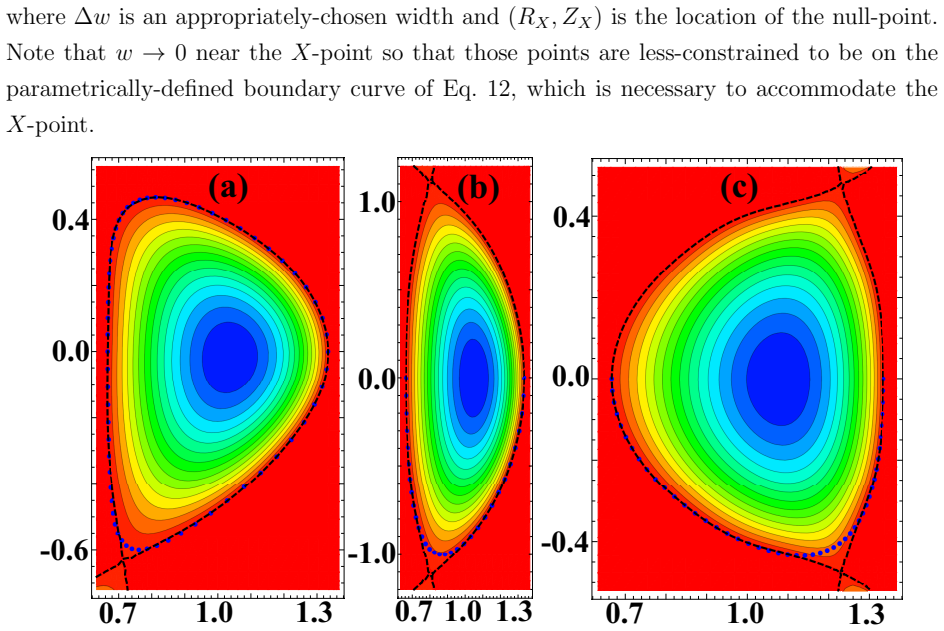
The machinery is the constrained least-squares system built from polynomial homogeneous solutions of $\Delta^*\psi=0$. The basis functions $P_i(R,Z)$ and $Q_i(R,Z)$, generated by the recursion $R\,\partial_R(R^{-1}\partial_R f_{i-2})=-i(i-1)f_i$, each satisfy the homogeneous equation identically, so any linear combination is an exact solution. Boundary constraints are assembled into the inner product $\langle p,q\rangle=\sum_j w_j\,p(R_j,Z_j)q(R_j,Z_j)$ over $M$ points on the parametric boundary curve, and the normal equations for the coefficients are solved in one matrix inversion. X-point constraints are enforced exactly by adding three Lagrange-multiplier rows and columns, with a Gaussian weight $w=1-e^{-[(R-R_X)^2+(Z-Z_X)^2]/\Delta_w^2}$ down-weighting boundary points near the null so that the exact null does not distort the boundary elsewhere.

What would settle it

For a fixed boundary shape, solve the least-squares system using $M$ sample points and then measure the maximum distance between the computed $\psi=0$ contour and the specified boundary on a much finer set of points; if that maximum error does not decrease as $M$ increases, or if it becomes large near X-points as the null constraints are added, the claimed decoupling of boundary accuracy from polynomial order is not working.

Watch

Extended reading notes

Core claim

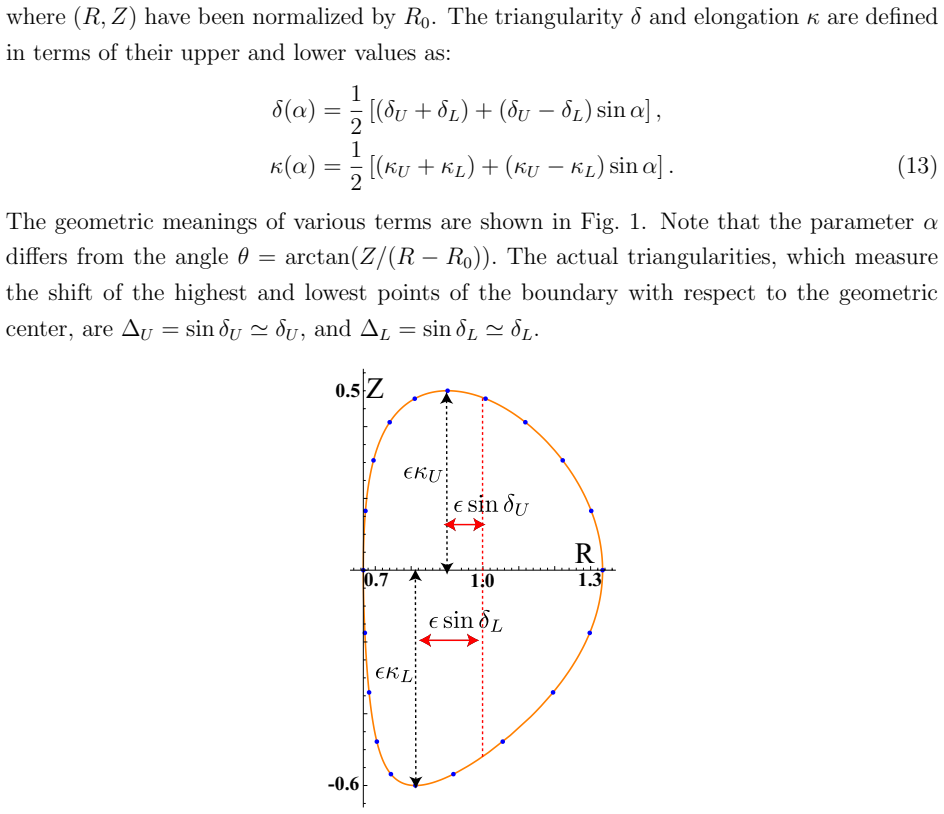
The central claim is that the fidelity of the boundary representation and the polynomial order of the homogeneous solution are decoupled. The flux function is written as $\psi=\psi_p+\psi_h$, where $\psi_p$ is a particular Solov'ev solution and $\psi_h$ is a finite polynomial solution of $\Delta^*\psi=0$. Instead of requiring the number of boundary constraints $M$ to equal the number of coefficients $N$, the paper imposes $\psi=0$ at $M\gg N$ points in a least-squares sense, and for X-point configurations adds the three null conditions $\psi=0$, $\partial\psi/\partial R=0$, $\partial\psi/\partial Z=0$ as exact constraints via Lagrange multipliers. Thus $M$ can be as large as the boundary specification demands while $N=2I$ (or $I$ for up-down symmetry) stays small, and $I$ is chosen only by how closely the computed boundary must follow the specified curve.

Load-bearing premise

The load-bearing premise is that a low-order polynomial solution fitted to many boundary points by least squares stays close to the specified boundary everywhere between those points, and that the Gaussian weighting near X-points does not degrade the fit elsewhere.

Editorial extensions

If this is right

Boundary specification no longer limits the analytic solution: users can add as many boundary points as they want while keeping the polynomial expansion small.
For up-down symmetric equilibria, only the even basis functions are needed and the constraints can be taken from half the boundary, halving the system size.
X-points enter as exact constraints rather than approximations, so single-null and double-null diverted configurations are handled in the same linear framework.
The resulting equilibria are exact analytic solutions of the linearized Grad-Shafranov equation and require only the inversion of a small linear system, making them convenient benchmarks for numerical equilibrium codes.
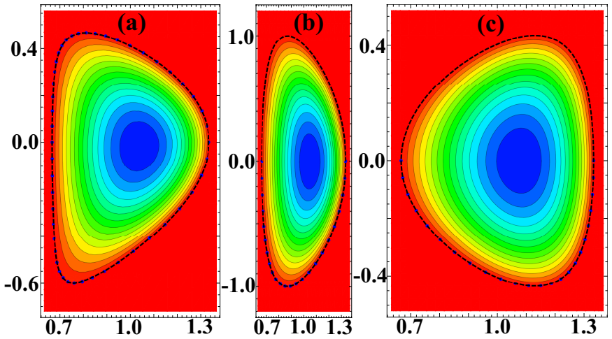
In the paper's examples, I=4 already gives acceptable results for the highly shaped fixed-boundary equilibria, and the displayed cases use M=4N.

Reading between the lines

Editorial extensions of the paper, not claims the author makes directly.

The same least-squares decoupling should transfer to other linear elliptic equations with known homogeneous solution families, though the paper does not explore that extension.
A natural robustness test not reported in the paper is the condition number of the normal matrix as $M$ and $I$ grow; ill-conditioning would limit how large $M$ can usefully become.
Because each boundary costs only one small linear solve, the method could generate exact equilibria in batches for scans over shape parameters, which would suit optimization or uncertainty studies.

Share X Bluesky LinkedIn Reddit HN

Signed reviews

No signed human review yet.

Editorial analysis

A structured set of objections, weighed in public.

Desk editor's note, referee report, and a circularity audit.

Desk Editor's Note

read the letter

Worth a look if you work with analytic equilibria for benchmarking. The new thing is simple and real: instead of matching M boundary points with M polynomial coefficients (the square system in Zheng and Cerfon-Freidberg), the authors solve an overdetermined least-squares problem with M>N, and impose X-point constraints exactly with Lagrange multipliers. The math in Eqs. (16)-(25) is correct, and the examples in Figs. 2-3 show that modest polynomial orders (I=6-12) handle quite shaped boundaries. The appendix polynomials are a useful resource, and implementation is straightforward.

The soft spots are mostly about the claims, not the derivation. The abstract says the boundary can be specified with 'arbitrarily large number of constraints' and that the polynomial order becomes independent of boundary accuracy. That's only half true. For fixed I, the homogeneous solution is an N-dimensional family of flux functions. Adding more M refines the discrete sampling of that family, but it cannot reduce the boundary error below the distance from the target curve to the family. So I and boundary complexity are still coupled; the paper just makes the coupling less direct. The examples demonstrate this in practice, but they don't measure it.

The numerical validation is also thinner than I'd like. No residuals, no convergence study in I, no conditioning numbers. The figures are self-consistency checks on the same points used for the fit. The X-point case has an additional open knob: the Gaussian weight width Δw in Eq. (26) is 'appropriately chosen' but never specified, and the near-X-point boundary is deliberately not controlled. The size of that uncontrolled region is unknown.

For a methods paper this is a solid, citable contribution. It doesn't need new physics to be useful. But the abstract should be toned down, and a revision should include an error metric and a small convergence study. I would send it to review.

Referee Report

3 major / 6 minor

Summary. This paper presents a constrained least-squares method for constructing exact Solov'ev equilibria, i.e., solutions of the Grad-Shafranov equation with linear source functions, whose plasma boundary is specified by a parametric curve. The boundary is enforced by minimizing the sum of squared residuals of the flux at a large number of points (M) relative to the number of degrees of freedom (N) in the homogeneous polynomial solution, and X-point constraints are imposed exactly using Lagrange multipliers. Three fixed-boundary and three diverted equilibria are shown as examples. The central claims are that the boundary specification can be decoupled from the polynomial expansion order and that arbitrarily many boundary constraints can be used while keeping N small.

Significance. If the decoupling claim were fully substantiated, the method would be a convenient tool for generating analytic equilibria for benchmarking and stability studies. The derivation of the normal equations and the constrained system is clear, the polynomial basis is provided explicitly, and the examples demonstrate that the approach is computationally cheap and easy to implement. However, the over-arching claim about arbitrary boundaries with fixed N is only partially true, and the quantitative support for boundary fidelity in the examples is missing; these gaps should be addressed before the method can be used with confidence for strongly shaped or diverted boundaries.

major comments (3)

[§II.C, Eqs. (10), (15)–(17)] The central claim that the boundary definition can be decoupled from the size N of the homogeneous solution is not established as stated. For fixed I, Eq. (10) spans an N-dimensional linear space, and the set of attainable zero-level boundaries is an N-parameter family; the least-squares solution of Eqs. (16)–(17) is the projection of the target boundary samples onto that family. Enlarging M only refines the sampling of this projection and cannot reduce the approximation error below the distance from the target curve to the family. The paper shows no residual magnitudes, no convergence study as I is increased, and no conditioning information for the normal equations, so the abstract's claim that 'an arbitrarily large number of constraints' ensures accurate representation requires qualification: I must also grow with the boundary complexity.
[§II.D, Eq. (26), Fig. 3] The Gaussian weight (26) intentionally de-emphasizes boundary points near an X-point, so the separatrix shape there is controlled by the X-point constraints and the polynomial expansion, not by the specified boundary. The extent of the uncontrolled region is determined by Δ_w, which is described only as 'appropriately chosen'; the paper gives no guidance or sensitivity analysis for this parameter. Since the visible deviations in Fig. 3 are near the X-points, a user cannot infer an accuracy guarantee for the boundary representation in diverted configurations.
[§II.D, Eqs. (19)–(25)] The paper claims applicability to configurations with 'one or more X-points,' but Section II.D formulates the Lagrange-multiplier procedure for a single (R_X, Z_X) only. The double-null example in Fig. 3(b) presumably requires two sets of constraints, and the manuscript does not explain how additional multiplier sets are appended or how potential inconsistency between multiple X-point constraints is handled. This omission is significant because the constraint system must be satisfied exactly for each X-point.

minor comments (6)

[§II.B, text near Eq. (14)] The sentence 'there are obvious advantageous to having M≫N' should read 'advantages'; moreover, the examples use M=4N, which is not '≫' as the text suggests.
[§II.C, Eq. (15)] The particular solution is denoted ψ_p in Eq. (7) but ψP in Eq. (15); the notation should be unified.
[§II.D, Eq. (26)] The values of Δ_w used in the examples are not reported; at minimum, the paper should list these values and state the sensitivity of the computed boundary to this choice.
[Figures 2 and 3] The figures show only visual agreement between the specified points and the computed boundary; plotting the residual as a function of the parameter α would provide a much more informative measure of the method's accuracy, especially between sample points.
[Appendix] The statement that 'P_{I-1} has order I, while Q_I has order I+1' is potentially confusing because I is used both as a maximum index and as the polynomial order; a short explanation of the indexing convention would help.
[References] Reference [6] is listed as 'submitted for publication' without a journal name; this should be updated or completed before publication.

Circularity Check

0 steps flagged · score 0.0 of 10

No significant circularity: the boundary fit is a construction, not a prediction, and the equilibrium solution is verified by direct substitution.

full rationale

The paper's derivation is self-contained. It takes the linear Solov'ev equation (Eq. 3), combines a particular solution (Eq. 7) with a homogeneous polynomial basis (Eq. 10), and determines the coefficients by minimizing a residual sum (Eq. 15), with X-point constraints imposed exactly via Lagrange multipliers (Eqs. 20-25). The basis polynomials are listed in the Appendix and can be checked by direct substitution, so the solution satisfies the equilibrium equation exactly. The agreement between the specified boundary points and the computed zero contour in Figs. 2 and 3 is a consistency check by construction: those points are exactly the data used to determine the coefficients. This is not circular because the paper does not present that agreement as an independent prediction; it presents the method as a construction of exact Solov'ev equilibria. The only self-citation (Ref. 6) is a passing reference to the authors' earlier free-boundary method and is not load-bearing. The claim that the boundary specification is decoupled from the polynomial order is a technical accuracy limitation: for fixed I the attainable zero sets form an N-parameter family, and increasing M cannot reduce the approximation error below the distance from the target curve to that family. That is a correctness or conditioning concern, not a circularity, because no fitted quantity is renamed as a prediction and no result is assumed from prior work by the same authors to force the solution form.

Assumptions & free parameters 3 free parameters · 4 assumptions · 0 invented entities

The construction is self-contained; free parameters are methodological choices (I, M, and the X-point weight width) rather than fitted physics. The main unproved axiom is finite-polynomial approximability of arbitrary boundaries, which is supported only by visual examples.

free parameters (3)

Polynomial truncation order I = varies (I=6 for fixed-boundary examples; I=8 and I=12 for X-point examples)
The order of the homogeneous polynomial expansion is chosen by hand per example and directly controls how closely the boundary can be fit. The paper gives no automatic criterion for choosing I.
Number of boundary constraints M = M=4N in all examples
M is a user choice; larger M samples the boundary more finely but changes the least-squares system. No convergence study is provided.
Gaussian weight width Delta_w in Eq. 26 = not given
For X-point equilibria, the weight that de-emphasizes points near the null has an 'appropriately chosen' width. No value or selection rule is reported, yet the resulting boundary depends on it.

assumptions (4)

domain assumption The axisymmetric equilibrium is governed by the Grad-Shafranov equation (Eq. 1).
The entire construction models tokamak equilibria within ideal MHD; if this equation does not apply, the result does not apply.
domain assumption The source functions are restricted to linear Solov'ev forms, with mu0 p' = -C and FF' = -A R0^2 (Eq. 3).
This linearization is what makes the PDE linear and the solutions 'exact'; general p(psi) and F(psi) are outside the method.
domain assumption A truncated polynomial basis (Eq. 10 with finite I) can represent the specified boundary accurately.
The claim of arbitrary boundaries rests on this approximation property, but no convergence or error bound is shown; only examples are given.
ad hoc to paper The Gaussian weight (Eq. 26) that de-emphasizes points near X-points preserves boundary fidelity elsewhere.
The weight is introduced without a derivation, and its width is 'appropriately chosen'; the results depend on it.

how reviews work

0 comments

Cite this review

Pith. "Pith review of Exact Solov'ev equilibrium with an arbitrary boundary." pith.science (2026). https://pith.science/paper/IPI54RBJ

@misc{pith2026190804449,
  author       = {Pith},
  title        = {Pith review of: Exact Solov'ev equilibrium with an arbitrary boundary},
  year         = {2026},
  howpublished = {\url{https://pith.science/paper/IPI54RBJ}},
  note         = {Machine review of arXiv:1908.04449}
}

abstract

Exact Solov'ev equilibria for arbitrary plasma cross-sections are calculated using a constrained least-squares method. The boundary, with or without $X$-points, can be specified with an arbitrarily large number of constraints to ensure an accurate representation. Thus, the order of the polynomial basis functions in the homogeneous solution of the Grad-Shafranov equation becomes an independent parameter determined only by the accuracy requirements of the overall solution. Examples of exact, highly-shaped equilibria are presented.

Figures

Figures reproduced from arXiv: 1908.04449 by the authors.

**Figure 2.** FIG. 2 [PITH_FULL_IMAGE:figures/full_fig_p007_2.png] view at source ↗

**Figure 3.** FIG. 3 [PITH_FULL_IMAGE:figures/full_fig_p009_3.png] view at source ↗

Discussion (0). Continue with ORCID to comment.

Reference graph

Works this paper leans on

16 extracted references · 16 canonical work pages

[1]

Grad and author H

author H. Grad and author H. Rubin , in booktitle Proceedings of the Second United Nations Conference on the Peaceful Uses of Atomic Energy ( publisher United Nations , address Geneva , year 1958 )

work page 1958
[2]

author V. D. Shafranov , journal Zh. Teor. Fiz. volume 33 , pages 710 ( year 1957 ), note [Sov. Phys. - JETP 6, 545 (1958)]

work page 1958
[3]

Jardin , title Computational Methods in Plasma Physics ( publisher CRC Press , address Boca Raton, FL , year 2010 )

author S. Jardin , title Computational Methods in Plasma Physics ( publisher CRC Press , address Boca Raton, FL , year 2010 )

work page 2010
[4]

Freidberg , title Ideal MHD ( publisher Cambridge University Press , address Cambridge, UK , year 2014 )

author J. Freidberg , title Ideal MHD ( publisher Cambridge University Press , address Cambridge, UK , year 2014 )

work page 2014
[5]

Takeda and author S

author T. Takeda and author S. Tokuda , journal J. Comp. Phys. volume 93 , pages 1 ( year 1991 )

work page 1991
[6]

author K. S. Han , author B. H. Park , author A. Y. Aydemir , and author J. Ko , journal submitted for publication to J. Comput. Phys. ( year 2019 )

work page 2019
[7]

L \"u tjens , author A

author H. L \"u tjens , author A. Bondeson , and author O. Sauter , journal Comp. Phys. Commun. volume 97 , pages 219 ( year 1996 )

work page 1996
[8]

author L. L. Lao , author H. E. St. John , author Q. Peng , author J. R. Ferron , author E. J. Strait , author T. S. Taylor , author W. H. Meyer , author C. Zhang , and author K. I. You , journal Fusion Science and Technology volume 48 , pages 968 ( year 2005 )

work page 2005

Show all 16 references

[9]

author P. J. McCarthy , journal Phys. Plasmas volume 6 , pages 3554 ( year 1999 )

1999
[10]

author C. V. Atanasiu , author S. Günter , author K. Lackner , and author I. G. Miron , journal Phys. Plasmas volume 11 , pages 3510 ( year 2004 )

2004
[11]

Guazzotto and author J

author L. Guazzotto and author J. P. Freidberg , journal Phys. Plasmas volume 14 , pages 112508 ( year 2007 )

2007
[12]

author L. S. Solov'ev , journal Zh. Teor. Fiz. volume 53 , pages 626 ( year 1967 ), note [Sov. Phys. - JETP 26, 400 (1968)]

1968
[13]

author M. F. Reusch and author G. H. Nielson , journal J. Comp. Phys. volume 64 , pages 416 ( year 1986 )

1986
[14]

author S. B. Zheng , author A. J. Wootton , and author E. R. Solano , journal Phys. Plasmas volume 3 , pages 1176 ( year 1996 )

1996
[15]

author A. J. Cerfon and author J. P. Freidberg , journal Phys. Plasmas volume 17 , pages 032502 ( year 2010 )

2010
[16]

, title Mathematica, V ersion 12.0 , note Champaign, IL, 2019

author Wolfram Research , Inc. , title Mathematica, V ersion 12.0 , note Champaign, IL, 2019

2019

Pith tools

Reviewed August 14, 2026 · model on record in the stance chip above.

[1] [1]

Grad and author H

author H. Grad and author H. Rubin , in booktitle Proceedings of the Second United Nations Conference on the Peaceful Uses of Atomic Energy ( publisher United Nations , address Geneva , year 1958 )

work page 1958

[2] [2]

author V. D. Shafranov , journal Zh. Teor. Fiz. volume 33 , pages 710 ( year 1957 ), note [Sov. Phys. - JETP 6, 545 (1958)]

work page 1958

[3] [3]

Jardin , title Computational Methods in Plasma Physics ( publisher CRC Press , address Boca Raton, FL , year 2010 )

author S. Jardin , title Computational Methods in Plasma Physics ( publisher CRC Press , address Boca Raton, FL , year 2010 )

work page 2010

[4] [4]

Freidberg , title Ideal MHD ( publisher Cambridge University Press , address Cambridge, UK , year 2014 )

author J. Freidberg , title Ideal MHD ( publisher Cambridge University Press , address Cambridge, UK , year 2014 )

work page 2014

[5] [5]

Takeda and author S

author T. Takeda and author S. Tokuda , journal J. Comp. Phys. volume 93 , pages 1 ( year 1991 )

work page 1991

[6] [6]

author K. S. Han , author B. H. Park , author A. Y. Aydemir , and author J. Ko , journal submitted for publication to J. Comput. Phys. ( year 2019 )

work page 2019

[7] [7]

L \"u tjens , author A

author H. L \"u tjens , author A. Bondeson , and author O. Sauter , journal Comp. Phys. Commun. volume 97 , pages 219 ( year 1996 )

work page 1996

[8] [8]

author L. L. Lao , author H. E. St. John , author Q. Peng , author J. R. Ferron , author E. J. Strait , author T. S. Taylor , author W. H. Meyer , author C. Zhang , and author K. I. You , journal Fusion Science and Technology volume 48 , pages 968 ( year 2005 )

work page 2005