REVIEW 3 major objections 4 minor 91 references
Homogeneously derived transit timings for 17 exoplanets and reassessed TTV trends for WASP-12 and WASP-4
T0 review · 3 major / 4 minor · reviewed 2026-08-14 · deepseek-v4-flash
Pith's one-line read WASP-12 shows a genuine quadratic transit-timing trend, but about 10% of it is a light-travel (Roemer) effect; the truly tidal decay time is 3.80 ± 0.40 Myr, while WASP-4's claimed trend is model-dependent.
desk verdict Solid homogeneous TTV study that confirms WASP-12's TTV trend, but the ~10% Roemer correction rests on a ~1-sigma RV choice; WASP-4 skepticism is well founded. read the letter →
The pith
A machine-rendered reading of the paper's core claim, the machinery that carries it, and where it could break.
The reading
What carries the argument
The argument is carried by a quadratic transit-timing model $TTV(t)=T_0+(t-t_0)-(t-t_0)^2/(2T_d)$, where $T_d=-P/\dot P$ is the apparent period-decay time, together with the identity $T_d^{RA} = 300/c_1$ (with $c_1$ in m/s/yr giving $T_d$ in Myr), which converts a radial acceleration into an equivalent Roemer light-travel decay time. Subtracting $1/T_d^{RA}$ from $1/T_d$ isolates the tidal part. Around this, the paper builds a homogeneous pipeline: all ~1,100 lightcurves are reprocessed with the same red-noise model, the same quadratic limb-darkening law, and empirically debiased limb-darkening coefficients, then fitted jointly with archival radial velocities, including Rossiter–McLaughlin corrections.
What would settle it
Take new high-precision radial velocities of WASP-12 over the next several years: if the -7.5 ± 2.2 m/s/yr acceleration does not persist as a stable linear trend, the Roemer correction collapses and the tidal decay time returns to the apparent ~3.47 Myr. For WASP-4, a second season of homogeneous transits and simultaneous radial-velocity monitoring can decide whether any quadratic term remains once the four external transmission-spectroscopy timings are excluded.
Extended reading notes
Core claim
The central discovery is that a homogeneous, uniformly reprocessed transit-timing sample, combined with Doppler measurements, can separate genuine tidal orbital decay from light-travel artifacts. In WASP-12 the quadratic TTV trend is real and robust, with apparent decay time $T_d = 3.47\pm0.32$ Myr. Because the radial velocities show an acceleration $c_1 = -7.5\pm2.2$ m/s/yr, part of this apparent decay is a Roemer delay induced by a distant companion; subtracting the corresponding inverse decay time yields the truly tidal value $T_d^{tidal} = 3.80\pm0.40$ Myr. In WASP-4, the quadratic trend reported by a recent TESS-based analysis is not reproduced by the homogeneous data alone, and its significance depends heavily on four externally published timings and on how heterogeneous TTV noise is modelled, so the trend's existence and magnitude remain uncertain.
Load-bearing premise
The 10 per cent Roemer correction and the revised 3.80 Myr tidal time rest on the assumption that the measured -7.5 ± 2.2 m/s/yr radial acceleration is a real line-of-sight acceleration from an unseen companion, not red noise or an instrument artifact.
Editorial extensions
If this is right
- WASP-12's orbit is decaying by tides, and the true decay time is about 10 per cent longer than the raw TTV trend suggests; tidal quality factor estimates based on the uncorrected value are slightly too aggressive.
- Unseen companions can masquerade as apparent tidal decay in TTV data; any future TTV trend detection should be checked against Doppler accelerations before interpreting it as orbital decay.
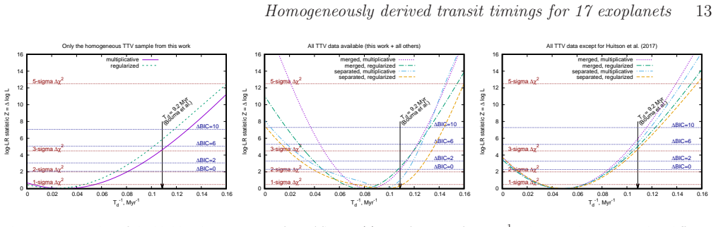
- WASP-4's claimed TTV trend is not robust: the homogeneous sample is consistent with a linear ephemeris, and removing four external timings reduces the significance to about 3 sigma, so it cannot yet be used to constrain tidal physics.
- The empirical limb-darkening biases measured here, especially a roughly 0.1 shift in one of the quadratic coefficients, should be applied when reprocessing archival transit lightcurves, otherwise TTV noise is underestimated.
- Merging heterogeneous TTV data with adaptive weighting, rather than plain merging, can substantially change trend significances and should become standard practice.
Reading between the lines
- If the WASP-12 radial acceleration is confirmed by further Doppler monitoring, the unseen companion's orbit could be constrained jointly from the TTV and RV signals, turning a nuisance into a discovery.
- The WASP-4 case suggests that other published TTV trend claims based on mixed-quality timings may lose significance when reanalysed with separately weighted noise models; revisiting such claims could reveal a broader class of marginal detections.
- The 10 per cent Roemer correction implies that TTV-only estimates of tidal decay times for hot Jupiters may be systematically biased by roughly that amount, which is comparable to current 1-sigma uncertainties and could matter for theory comparisons.
- A practical extension would be to apply the same homogeneous reprocessing to much larger archival samples, since the pipeline's power comes from removing inter-team biases rather than from any single new observation.
Signed reviews
Editorial analysis
A structured set of objections, weighed in public.
Referee Report
Summary. The paper presents a homogeneous re-analysis of roughly 1100 transit light curves for 17 exoplanet hosts, combining archival and new EXPANSION photometry with radial-velocity data for 13 targets. The authors derive transit timings with a common pipeline, empirically calibrate limb-darkening coefficients, and fit self-consistent transit-plus-RV models. Their main results are: (i) a high-significance (about 9-sigma) quadratic TTV trend in WASP-12, consistent with previous work and cross-checked against independent Maciejewski et al. timings; (ii) hints of a radial acceleration of approximately -7.5 +/- 2.2 m/s/yr for WASP-12, implying that roughly 10% of the apparent TTV is a Roemer effect and that the truly tidal decay time is T_tidal = 3.80 +/- 0.40 Myr; and (iii) a demonstration that the WASP-4 TTV trend reported by Bouma et al. is model-dependent, disappearing in the homogeneous sample and dropping to 2.8-3 sigma when the four Huitson et al. timings are removed. The paper also reports no significant periodic TTVs in the other targets and provides revised transit parameters and RV trends.
Significance. The paper's main strength is its careful attention to data homogeneity: the same pipeline and noise model are applied to all light curves, and the quantitative comparison with independent Maciejewski et al. timings for WASP-12 (12% RMS difference) provides a credible external validation. The empirical limb-darkening calibration and the likelihood-ratio analysis for WASP-4 are useful methodological contributions. If the WASP-12 radial acceleration is real, the Roemer correction would be an important new ingredient in interpreting this famous tidal-decay candidate, with consequences for the inferred tidal quality factor. The WASP-4 analysis is a valuable cautionary counterpoint to the earlier detection claim, and the release of the reprocessed photometry and derived timings is a community resource. The main caveats, which the authors themselves partly identify, concern the statistical support for the preferred RV fit in Section 7 and the conditional nature of the WASP-4 significance after subset removal; these points need to be addressed in revision.
major comments (3)
- [Section 7, Eq. (12), Table 5] The claimed 'roughly 10 per cent' Roemer correction is based on choosing the 'alternative' fit WASP-12' with c1 = -7.5 +/- 2.2 m/s/yr over the split-RV fit WASP-12 with c1 = -5.4 +/- 2.0 m/s/yr. The paper justifies this preference only qualitatively, by arguing that local red noise in short in-transit runs may contaminate the basic fit, and it gives no statistical model comparison (BIC/AIC or a formal test for local red noise). The two c1 values differ by less than one sigma. Propagating c1 = -5.4 through Eq. (12) gives T_tidal = 3.70 +/- 0.38 Myr instead of 3.80 +/- 0.40 Myr. The raw TTV detection is robust regardless of this choice, but the specific '~10 per cent larger' statement in the abstract and Section 7 is model-dependent; it should be supported by a quantitative comparison of the two fits or softened to a range that covers both values.
- [Section 5.5, Fig. 4] The 2.8-3 sigma significance quoted after removing the four Huitson et al. timings is computed from a merged compilation of heterogeneous TTV datasets. This is in tension with the paper's own central methodological warning that heterogeneous TTV data should not be plainly merged. The significance therefore measures the trend under a particular ad hoc subset and merging model, not on the homogeneous sample. The paper should state explicitly that this 2.8-3 sigma value is conditional on the adopted subset and noise model, and it should present the homogeneous-sample upper limit as the primary WASP-4 result. As written, a reader may overinterpret the 2.8-3 sigma as a robust estimate of the trend's significance.
- [Sections 5.1 and 5.5] The paper demonstrates in Section 5.1 that its own TTV uncertainties are underestimated by about 22 per cent for WASP-12 (reduced chi^2 = 1.49) and applies this correction in Section 5.4. It is not stated whether the WASP-4 homogeneous-sample significance limits in Fig. 4 include an analogous correction for WASP-4's reduced chi^2 = 1.31 from Table 2. If they do not, the statement that the homogeneous WASP-4 data are consistent with a linear ephemeris 'below 1-sigma' may be overconfident. The authors should specify whether the jitter and regularization parameters used in Fig. 4 were fit from the TTV residuals and, if so, quote the significance with and without the chi^2-based scaling.
minor comments (4)
- [Abstract and Section 5.5] There are typographical errors: 'homogeneus' should be 'homogeneous' in the abstract, and 'Peridograms' should be 'Periodograms' in Section 5.2.
- [Section 5.1] The statement that the 12 per cent RMS difference between the two WASP-12 TTV series is comparable to the 'probable statistical uncertainty (1/sqrt(N) for N=73)' is imprecise; the uncertainty of a ratio of two RMS estimates is more like sqrt(2/(N-1)) ~ 17 per cent. Please rephrase to avoid giving a misleading uncertainty estimate.
- [Section 4] The text says the 'Clear' band limb-darkening coefficients are always fitted, but the comparison with bolometric values in Figs 3 and 4 is said to be for reference only. It would be helpful to state explicitly how the final pipeline treats the Clear band, since this band includes many amateur light curves.
- [Section 2, Table 1] For Qatar-2, the assumption that the published 'BJD' times are in the TDB system is justified only by the statement that the TTV residuals look bad otherwise; the footnote could quantify how much the alternative UTC interpretation changes the derived timings, to make the assumption more transparent.
Circularity Check
No significant circularity: the TTV trend and the Roemer correction rest on independent observables.
full rationale
The WASP-12 quadratic TTV term is measured directly from the homogeneously reprocessed transit times (Fig. 2) and is cross-checked against the independent Maciejewski et al. (2016, 2018b) timings in Sect. 5.1, where both series give nearly identical trend fits. The radial acceleration c1 is derived from a separate observable, the Doppler data, and is not fitted to the TTV residuals; the Roemer decomposition in Eqs. (10)-(12) is a physical subtraction of two independently measured quadratic coefficients rather than an identity imposed by the model. The only judgment-sensitive step, preferring the WASP-12' RV fit with c1 = -7.5 m/s/yr over the split-RV value c1 = -5.4 m/s/yr, is explicitly presented as a belief rather than a statistical test, and the resulting ~10% correction is within the quoted 1-sigma uncertainty, so it does not constitute a forced prediction. The empirical limb-darkening bias calibration in Sect. 4 is a nuisance-parameter correction applied to the same lightcurves, but the target quantity, the long-term TTV trend, is not defined in terms of those biases and remains stable against the external comparison. For WASP-4, the paper's central claim is that the trend significance is model-dependent, which is a sensitivity analysis rather than a circular derivation. Self-citations to Baluev (2009, 2015, 2018) provide algorithms and software, but they are not invoked as the sole support for any scientific conclusion and do not make the derivation equivalent to its inputs.
Assumptions & free parameters
free parameters (5)
- WASP-12 TTV decay time Td =
3.47 +/- 0.32 Myr
- WASP-12 radial acceleration c1 =
-7.5 +/- 2.2 m/s/yr
- Limb-darkening bias corrections =
Delta A = 0.004 +/- 0.008, Delta B = -0.099 +/- 0.014
- Shared red-noise timescale tau =
not quoted; range about 10 sec to 50 min, typically 1-5 min
- TTV jitter for WASP-12 =
20.8 +/- 2.5 sec
assumptions (6)
- domain assumption Quadratic TTV model (Eq. 5) can represent tidal decay, apsidal precession, or Roemer effect
- domain assumption Roemer effect relation Td = C/c1 (Eq. 11)
- standard math Quadratic limb-darkening law (Eq. 1) with monotonicity constraints
- domain assumption Statistical independence of TTV trend and RV trend coefficients
- ad hoc to paper Exponential-correlation Gaussian process red noise model and its detection criteria
- domain assumption Stellar masses in Table 4 are fixed and their uncertainties ignored
invented entities (1)
-
Unseen distant companion(s) around WASP-12
Cite this review
Pith. "Pith review of Homogeneously derived transit timings for 17 exoplanets and reassessed TTV trends for WASP-12 and WASP-4." pith.science (2026). https://pith.science/paper/MHFTRQR4
@misc{pith2026190804505,
  author       = {Pith},
  title        = {Pith review of: Homogeneously derived transit timings for 17 exoplanets and reassessed TTV trends for WASP-12 and WASP-4},
  year         = {2026},
  howpublished = {\url{https://pith.science/paper/MHFTRQR4}},
  note         = {Machine review of arXiv:1908.04505}
}
abstract
We homogeneously analyse $\sim 3.2\times 10^5$ photometric measurements for $\sim 1100$ transit lightcurves belonging to $17$ exoplanet hosts. The photometric data cover $16$ years 2004--2019 and include amateur and professional observations. Old archival lightcurves were reprocessed using up-to-date exoplanetary parameters and empirically debiased limb-darkening models. We also derive self-consistent transit and radial-velocity fits for $13$ targets. We confirm the nonlinear TTV trend in the WASP-12 data at a high significance, and with a consistent magnitude. However, Doppler data reveal hints of a radial acceleration about $(-7.5\pm 2.2)$~m/s/yr, indicating the presence of unseen distant companions, and suggesting that roughly $10$ per cent of the observed TTV was induced via the light-travel (or Roemer) effect. For WASP-4, a similar TTV trend suspected after the recent TESS observations appears controversial and model-dependent. It is not supported by our homogeneus TTV sample, including $10$ ground-based EXPANSION lightcurves obtained in 2018 simultaneously with TESS. Even if the TTV trend itself does exist in WASP-4, its magnitude and tidal nature are uncertain. Doppler data cannot entirely rule out the Roemer effect induced by possible distant companions.
Figures


Figures from the paper (1 more)
Reference graph
Works this paper leans on
-
[1]
C., 2017, in Deeg H
Agol E., Fabrycky D. C., 2017, in Deeg H. J., Belmonte J. A., eds, , Handbook of Exoplanets. Springer, Cham
2017
-
[2]
Albrecht S., et al., 2012, , 757, 18
2012
-
[3]
Alonso R., et al., 2008, , 482, L21
2008
-
[4]
P., 2012, , 200, 15
Anglada-Escud\'e G., Butler R. P., 2012, , 200, 15
2012
-
[5]
Bailey A., Goodman J., 2019, , 482, 1872
2019
-
[6]
A., et al., 2006, , 650, 1160
Bakos G. A., et al., 2006, , 650, 1160
2006
-
[7]
A., et al., 2009, , 707, 446
Bakos G. A., et al., 2009, , 707, 446
2009
-
[8]
V., 2008, , 385, 1279
Baluev R. V., 2008, , 385, 1279
2008
Show all 91 references
-
[9]
V., 2009, , 393, 969
Baluev R. V., 2009, , 393, 969
2009
-
[10]
V., 2013, Astron
Baluev R. V., 2013, Astron. & Comp., 2, 18
2013
-
[11]
V., 2015, , 446, 1493
Baluev R. V., 2015, , 446, 1493
2015
-
[12]
V., 2018, Astron
Baluev R. V., 2018, Astron. & Comp., 25, 221
2018
-
[13]
V., Shaidulin V
Baluev R. V., Shaidulin V. S., 2015, , 454, 4379
2015
-
[14]
V., et al., 2015, , 450, 3101
Baluev R. V., et al., 2015, , 450, 3101
2015
-
[15]
L., et al., 2008, , 486, 1039
Bean J. L., et al., 2008, , 486, 1039
2008
-
[16]
B., et al., 2014, , 788, 2
Bechter E. B., et al., 2014, , 788, 2
2014
-
[17]
G., et al., 2019, , 157, 217
Bouma L. G., et al., 2019, , 157, 217
2019
-
[18]
Brown A. G. A., Vallenari A., Prusti T., de Bruijne J. H. J., Babusiaux C., Bailer-Jones C. A. L., et al., 2018, , 616, A1
2018
-
[19]
L., et al., 2012, , 750, 84
Bryan M. L., et al., 2012, , 750, 84
2012
-
[20]
D., Minniti D., Naef D., Melo C., Mason E., Selman F., Pietrzynski G., 2009, , 507, 481
C\' a ceres C., Ivanov V. D., Minniti D., Naef D., Melo C., Mason E., Selman F., Pietrzynski G., 2009, , 507, 481
2009
-
[21]
N., Holman M
Chan T., Ingemyr M., Winn J. N., Holman M. J., Sanchis-Ojeda R., Esquerdo G., Everett M., 2011, , 141, 179
2011
-
[22]
Chen G., Pall\' e E., Nortmann L., Murgas F., Parviainen H., Nowak G., 2017, , 600, L11
2017
-
[23]
Claret A., 2000, , 363, 1081
2000
-
[24]
Claret A., 2004, , 428, 1001
2004
-
[25]
Claret A., Bloemen S., 2011, , 529, A75
2011
-
[26]
A., Kielkopf J
Collins K. A., Kielkopf J. F., Stassun K. G., 2017, , 153, 78
2017
-
[27]
Damasso M., et al., 2015, , 575, A111
2015
-
[28]
S., 2010, , 122, 935
Eastman J., Siverd R., Gaudi B. S., 2010, , 122, 935
2010
-
[29]
M., Holman M
Fernandez J. M., Holman M. J., Winn J. N., Torres G., Shporer A., Mazeh T., Esquerdo G. A., Everett M. E., 2009, , 137, 4911
2009
-
[30]
Foreman-Mackey D., Agol E., Ambikasaran S., Angus R., 2017, , 154, 220
2017
-
[31]
J., Shporer A., Winn J
Fulton B. J., Shporer A., Winn J. N., Holman M. J., P\' a l A., Gazak J. Z., 2011, , 142, 84
2011
-
[32]
Gillon M., et al., 2007, , 472, L13
2007
-
[33]
Gillon M., et al., 2009a, , 496, 259
-
[34]
Gillon M., et al., 2009b, , 501, 785
-
[35]
Gillon M., et al., 2010, , 511, A3
2010
-
[36]
Hebb L., et al., 2009, , 693, 1920
2009
-
[37]
Heyrovsk\' y D., 2007, , 656, 483
2007
-
[38]
Hoyer S., et al., 2013, , 434, 46
2013
-
[39]
M., D\' e sert J.-M., Bean J
Huitson C. M., D\' e sert J.-M., Bean J. L., Fortney J. J., Stevenson K. B., Bergmann M., 2017, , 154, 95
2017
-
[40]
B., 1952, , 116, 211
Irwin J. B., 1952, , 116, 211
1952
-
[41]
H., et al., 2019, , 483, 3781
Kasper D. H., et al., 2019, , 483, 3781
2019
-
[42]
M., 2013, , 435, 2152
Kipping D. M., 2013, , 435, 2152
2013
-
[43]
A., et al., 2014, , 785, 126
Knutson H. A., et al., 2014, , 785, 126
2014
-
[44]
C., Agol E., Williams B
Kundurthy P., Barnes R., Becker A. C., Agol E., Williams B. F., Gorelick N., Rose A., 2013, , 770, 36
2013
-
[45]
Maciejewski G., et al., 2010, , 407, 2625
2010
-
[46]
Maciejewski G., et al., 2013, , 551, A108
2013
-
[47]
Maciejewski G., et al., 2016, , 588, L6
2016
-
[48]
S., Maciejczak J., Puciata-Mroczynska M., Boulanger E., 2018a, Information Bulletin on Variable Stars, 63, 6243
Maciejewski G., Stangret M., Ohlert J., Basaran C. S., Maciejczak J., Puciata-Mroczynska M., Boulanger E., 2018a, Information Bulletin on Variable Stars, 63, 6243
-
[49]
Maciejewski G., et al., 2018b, Acta Astronomica, 68, 371
-
[50]
Mancini L., et al., 2014, , 443, 2391
2014
-
[51]
Mancini L., et al., 2017, , 465, 843
2017
-
[52]
Mancini L., et al., 2018, , 613, A41
2018
-
[53]
Mandel K., Agol E., 2002, , 580, L171
2002
-
[54]
R., Crouzet N., Deming D., Madhusudhan N., 2014, , 791, 55
McCullough P. R., Crouzet N., Deming D., Madhusudhan N., 2014, , 791, 55
2014
-
[55]
Montalto M., et al., 2012, , 427, 2757
2012
-
[56]
R., Damasso M., 2011a, , 527, A85
Nascimbeni V., Piotto G., Bedin L. R., Damasso M., 2011a, , 527, A85
-
[57]
R., Damasso M., Malavolta L., Borsato L., 2011b, , 532, A24
Nascimbeni V., Piotto G., Bedin L. R., Damasso M., Malavolta L., Borsato L., 2011b, , 532, A24
-
[58]
Nascimbeni V., et al., 2013, , 549, A30
2013
-
[59]
Nikolov N., Henning T., Koppenhoefer J., Lendl M., Masiejewski G., Greiner J., 2012, , 539, 159
2012
-
[60]
P\' a l A., et al., 2008, , 700, 783
2008
-
[61]
M., Szing A., Kiss L
P\' a l A., S\' a rneczky K., Szab\' o G. M., Szing A., Kiss L. L., Mez \"o G., Reg\' a ly Z., 2011, , 413, L43
2011
-
[62]
C., Winn J
Patra K. C., Winn J. N., Holman M. J., Yu L., Deming D., Dai F., 2017, , 154, 4
2017
-
[63]
P., Mauas P
Petrucci R., Jofr\'e E., Schwartz M., C\'uneo V., Mart\'inez C., G\'omez M., Buccino A. P., Mauas P. J. D., 2013, , 779, L23
2013
-
[64]
Pollacco D., et al., 2008, , 385, 1576
2008
-
[65]
Pont F., Zucker S., Queloz D., 2006, , 373, 231
2006
-
[66]
Pont F., et al., 2007, , 476, 1347
2007
-
[67]
Queloz D., et al., 2001, The Messenger, 105, 1
2001
-
[68]
M., 2014, , 147, 161
Ranjan S., Charbonneau D., D\' e sert J.-M., Madhusudhan N., Deming D., Wilkins A., Mandell A. M., 2014, , 147, 161
2014
-
[69]
N., Holman M
Sanchis-Ojeda R., Winn J. N., Holman M. J., Carter J. A., Osip D. J., Fuentez C. I., 2011, , 733, 127
2011
-
[70]
C., et al., 2013, , 556, A150
Santos N. C., et al., 2013, , 556, A150
2013
-
[71]
N., Holman M
Shporer A., Mazeh T., Pont F., Winn J. N., Holman M. J., Latham D. W., Esquerdo G. A., 2009, , 694, 1559
2009
-
[72]
J., et al., 2012, , 761, 123
Siverd R. J., et al., 2012, , 761, 123
2012
-
[73]
N., et al., 2018, , 480, 291
Sokov E. N., et al., 2018, , 480, 291
2018
-
[74]
Southworth J., 2015, Astrophysics Source Code Library, ascl:1511.016
2015
-
[75]
Southworth J., et al., 2009a, , 396, 1023
-
[76]
Southworth J., et al., 2009b, , 399, 287
-
[77]
Southworth J., et al., 2010, , 408, 1680
2010
-
[78]
Southworth J., Bruni I., Mancini L., Gregorio J., 2012, , 420, 2580
2012
-
[79]
B., Bean J
Stevenson K. B., Bean J. L., Seifahrt A., D\' e sert J.-M., Madhusudhan N., Bergmann M., Kreidberg L., Homeier D., 2014, , 147, 161
2014
-
[80]
M., et al., 2010, , 523, A84
Szab\' o G. M., et al., 2010, , 523, A84
2010
-
[81]
Torres G., 2007, , 671, L65
2007
-
[82]
N., Holman M
Torres G., Winn J. N., Holman M. J., 2008, , 677, 1324
2008
-
[83]
Tregloan-Reed J., et al., 2015, , 450, 1760
2015
-
[84]
Triaud A. H. M. J., et al., 2010, , 524, A25
2010
-
[85]
Tripathi A., et al., 2010, , 715, 421
2010
-
[86]
M., et al., 2008, , 675, L113
Wilson D. M., et al., 2008, , 675, L113
2008
-
[87]
N., et al., 2007a, , 133, 1828
Winn J. N., et al., 2007a, , 133, 1828
-
[88]
N., Holman M., Roussanova A., 2007b, , 657, 1098
Winn J. N., Holman M., Roussanova A., 2007b, , 657, 1098
-
[89]
N., Holman M., Carter J
Winn J. N., Holman M., Carter J. A., Torres G., Osip D. J., Beatty T., 2009, , 137, 3826
2009
-
[90]
N., et al., 2010, , 718, 575
Winn J. N., et al., 2010, , 718, 575
2010
-
[91]
T., 2005, , 117, 657
Wright J. T., 2005, , 117, 657
2005
Reviewed August 14, 2026 · model on record in the stance chip above.
Discussion (0). Continue with ORCID to comment.