REVIEW 1 major objections 6 minor 62 references
Uncertainty relation for the position of an electron in a uniform magnetic field from quantum estimation theory
T0 review · 1 major / 6 minor · reviewed 2026-08-14 · deepseek-v4-flash
Pith's one-line read The paper shows that estimating both position coordinates of an electron in a uniform magnetic field obeys a nontrivial uncertainty trade-off even though the position operators commute.
desk verdict A clean and honest model calculation showing that commuting position observables can have a non-trivial estimation-theoretic trade-off; the thermal-state transition is real but the gauge-independence claim stays unproved. read the letter →
The pith
A machine-rendered reading of the paper's core claim, the machinery that carries it, and where it could break.
The reading
What carries the argument
The load-bearing object is the mean square error matrix $V$ for the two parameters $\theta_1,\theta_2$ together with the two quantum Cramér–Rao inequalities. For any two-parameter model the inequality $V\ge G^{-1}$ yields component lower bounds and a product inequality involving $|\operatorname{Im} g_{12}|$, where $G^{-1}=[g_{ij}]$. The authors compute the SLD and RLD Fisher information matrices for the two unitary shift models; the imaginary off-diagonal part of the inverse Fisher information is what creates a trade-off between $V_{11}$ and $V_{22}$. In Model 2 the noncommuting mechanical momenta introduce a phase factor in the shifted wavefunction, which produces that imaginary off-diagonal term and hence the hyperbolic bound; in the pure-state Model 1 the term vanishes, so only independent component floors remain.
What would settle it
Prepare a thermal Landau electron with a known $\langle L\rangle_0$, estimate the two position shifts with unbiased measurements, and record the achievable mean square error pairs. The paper predicts that for $|\langle L\rangle_0|\le 1/2$ the SLD floor $V_{11},V_{22}\ge g_{11}^S$ is the relevant bound, while for $|\langle L\rangle_0|>1/2$ no estimator should enter the region below both the SLD lines and the RLD hyperbola. Finding a measurement with a mean square error pair below the predicted union of bounds would falsify the claim.
Extended reading notes
Core claim
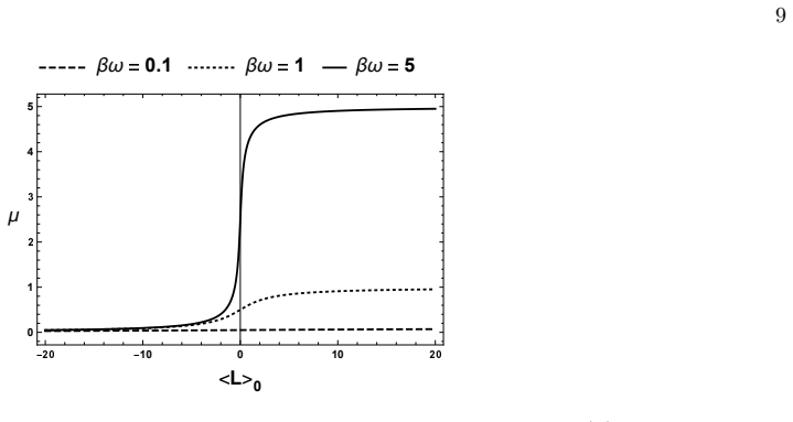
On the paper's own terms, the central discovery is that the mean square error matrix $V$ for estimating the two position-shift parameters is bounded by explicit quantum Cramér–Rao inequalities that depend on which momenta generate the shift. In the pure-state case the reference state is the $|0,0\rangle$ lowest Landau level with zero angular momentum. Model 1, generated by the commuting canonical momenta $p_x,p_y$, is quasi-classical: its SLD bound is $V_{11},V_{22}\ge \lambda^2/2$, and because its inverse Fisher information has no imaginary off-diagonal entry there is no trade-off between the two variances. Model 2, generated by the noncommuting mechanical momenta $\pi_x,\pi_y$, is a Gaussian shift model whose generalized RLD bound is $(V_{11}-\lambda^2/4)(V_{22}-\lambda^2/4)\ge \lambda^4/16$ and is achievable. With a thermal reference state constrained to fixed $\langle L\rangle_0$, Model 1's bound is determined by both the SLD and RLD inequalities: for $|\langle L\rangle_0|\le 1/2$ the SLD bound dominates, while for $|\langle L\rangle_0|>1/2$ both contribute and the bounds intersect twice; the bound is achievable only at $\langle L\rangle_0=0$. Model 2 remains a Gaussian shift model, so its RLD bound is achievable. The paper also shows that Model 2's bound is lower than Model 1's in both pure and thermal settings.
Load-bearing premise
The thermal-state analysis assumes that a degenerate thermal equilibrium is uniquely determined by fixing the expectation value of angular momentum with a chemical potential and that one root of the resulting equation is unphysical; if a preparation does not enforce this constraint, the derived bounds and the crossover at $|\langle L\rangle_0|=1/2$ need not apply.
Editorial extensions
If this is right
- Joint position estimation in a Landau system is limited by a genuine trade-off even though $X$ and $Y$ commute, so the Heisenberg–Robertson relation is not the right diagnostic for this sensing problem.
- The mechanical-momentum encoding (Model 2) gives a smaller, achievable Cramér–Rao bound than the canonical-momentum encoding in both pure and thermal regimes, so position measurements that exploit kinetic momentum can in principle be more accurate.
- In the thermal canonical-momentum model the uncertainty relation changes shape at $|\langle L\rangle_0|=1/2$, giving a signature of the angular momentum in the achievable estimation accuracy.
- For $\langle L\rangle_0\neq0$ the thermal Model 1 bound is not achievable, so optimal joint position estimation requires a strategy beyond separate position measurements; at $\langle L\rangle_0=0$ the SLD bound is achievable.
Reading between the lines
- Beyond the paper, the same estimation-theoretic construction should yield trade-offs for any pair of commuting observables that are linear combinations of noncommuting canonical variables; the Landau system is a concrete instance of a more general recipe.
- The crossover at $|\langle L\rangle_0|=1/2$ may reflect a qualitative change in the set of physical thermal preparations; a natural check is whether the same threshold appears in other degenerate harmonic-oscillator systems with a conserved angular momentum.
- Beyond the paper, the Model 2 advantage suggests an experimental direction: encode position information through kinetic-momentum displacements in a two-dimensional electron gas or a two-mode linear optical system, keeping in mind that the optimal measurement may require noncanonical variables.
Signed reviews
Editorial analysis
A structured set of objections, weighed in public.
Referee Report
Summary. This paper studies two-parameter quantum estimation of the position shift of a single electron in a uniform magnetic field, using either the canonical momenta (Model 1) or the mechanical momenta (Model 2) as displacement generators. For a pure lowest-Landau-level reference state, the authors derive quantum Cramér-Rao bounds for the mean-square-error matrix: Model 1 gives V11,V22 ≥ λ²/2 with no trade-off, while Model 2 gives (V11−λ²/4)(V22−λ²/4) ≥ λ⁴/16. For thermal reference states with a fixed expectation value of the angular momentum, Model 1 exhibits a bound determined by both the symmetric and right logarithmic derivative Cramér-Rao bounds, with a structural transition at |⟨L⟩0| = 1/2, and Model 2 is identified with a Gaussian shift model whose RLD bound is achievable. The paper concludes that quantum estimation theory can yield non-trivial uncertainty relations for two commuting observables.
Significance. If the technical issues below are resolved, the paper makes a useful conceptual contribution: it demonstrates explicitly that a trade-off relation for two commuting observables can arise from multi-parameter quantum estimation theory, in contrast to the Heisenberg-Robertson relation. The appendices provide detailed and largely checkable computations of the relevant Fisher information matrices, and the pure-state results are physically transparent. The authors are also careful to identify which bounds are achievable and which are not (e.g., Model 1 thermal bounds are not tight except at ⟨L⟩0 = 0). The thermal-state results are conditional on the explicit fixed-⟨L⟩0 grand-canonical ensemble, which is a stated modeling choice. The significance is moderate: the work is a clear application of known quantum estimation tools to a specific physical model, rather than a new general theorem.
major comments (1)
- [III A 2 and B 2 b] The matrix \tilde G^π_R reported in Appendix B 2 b is singular: det[[1,i],[-i,1]] = 0. Consequently ( \tilde G^π_R )^{-1} does not exist, and Eq. (29) cannot be the inverse of \tilde G^π_R as written. This affects the derivation of the central pure-state bound Eq. (30). The authors should clarify whether Eq. (29) is intended as a Moore-Penrose pseudoinverse and derive the bound accordingly, or present Eq. (30) as the zero-temperature limit of the thermal bound Eq. (51), which is non-singular for κ_a² > 0. The final inequality appears correct, but the derivation in the pure-state section is not.
minor comments (6)
- [II A] The assertion that the choice of gauge gives no change in the quantum Fisher information for a uniform magnetic field is stated without proof or reference; please provide a derivation or a citation.
- [IV A, Eq. (37)] The statement that one solution of Eq. (37) is unphysical because it gives a negative temperature state is not demonstrated; a short proof that the discarded branch violates μ>0 and βω>μ would strengthen the exposition.
- [IV B 1, Eq. (47)] The off-diagonal sign in the displayed matrix for (G_S)^{-1} − (G_R)^{-1} appears to be the opposite of what one obtains from the preceding explicit formulas; the condition |⟨L⟩0| ≤ 1/2 is unaffected, but the sign should be corrected.
- [Figure 1 caption] The caption's last sentence appears to confuse Model 1 and Model 2; please clarify which allowed region corresponds to which model.
- [IV C 1] The relation ξ2 = ξ*1 is inconsistent with Eq. (A10), where the second factor is e^{ξ* b† − ξ b}; either ξ2 = ξ or the expression should be adjusted.
- [Eq. (28)] The Gaussian exponent in Eq. (28) is missing parentheses; it should read exp[ −((x−θ1)² + (y−θ2)²)/λ² ].
Circularity Check
No significant circularity: the uncertainty relations are derived by direct application of standard quantum Cramér-Rao inequalities to explicit state families, with no fitted parameters renamed as predictions.
full rationale
The derivation chain is self-contained. The pure-state bounds (Eqs. (18)-(19), (29)-(30)) follow from computing SLD and generalized RLD Fisher information matrices for the explicit unitary shift models (3) and (6); the matrices are obtained by elementary operator algebra in Appendix B and are not fitted to any data. The thermal-state bounds (Eqs. (44)-(51)) likewise come from direct evaluation of RLD and SLD operators for the grand-canonical state (31) with fixed ⟨L⟩0; the chemical potential is solved from Eq. (37), and the transition at |⟨L⟩0|=1/2 is an algebraic consequence of the matrix inequality (G_S^{p thermal})^{-1} - (G_R^{p thermal})^{-1} ≥ 0. No parameter is estimated from a subset of data and then used to predict a closely related quantity. The self-citations ([27], [32], by one of the authors) are used only as external, independently published mathematical criteria for D-invariance and SLD achievability; the main lower bounds do not depend on them, and the paper explicitly discloses where its bounds are not tight (Model 1 thermal case, except ⟨L⟩0=0). Identification of Model 2 with the known Gaussian shift model is a stated reduction to an existing result, not a circular renaming. Accordingly, no load-bearing circular step was found.
Assumptions & free parameters
assumptions (5)
- domain assumption The symmetric gauge A = B(-y/2, x/2, 0) is adopted, and gauge choice is claimed not to affect quantum Fisher information (Sec. II A).
- domain assumption Ladder operators a,b and vacuum state |0,0> describe the lowest Landau level with zero angular momentum (Secs. II A-II B).
- standard math The Baker-Campbell-Hausdorff formula and Gaussian phase-space integrals are used to evaluate shifts and thermal states (Eqs. (26), (35), (B5)).
- standard math Existence and properties of SLD, RLD, and generalized RLD Fisher information and the D-invariance achievability criterion are taken from Fujiwara-Nagaoka, Suzuki, Yuen-Lax.
- ad hoc to paper The thermal state is fixed by the constraint <L>0 = constant through a chemical potential μ, and the physically relevant solution of Eq. (37) is selected (Sec. IV A).
Cite this review
Pith. "Pith review of Uncertainty relation for the position of an electron in a uniform magnetic field from quantum estimation theory." pith.science (2026). https://pith.science/paper/N4DK5BDM
@misc{pith2026190804868,
  author       = {Pith},
  title        = {Pith review of: Uncertainty relation for the position of an electron in a uniform magnetic field from quantum estimation theory},
  year         = {2026},
  howpublished = {\url{https://pith.science/paper/N4DK5BDM}},
  note         = {Machine review of arXiv:1908.04868}
}
read the original abstract
We investigate the uncertainty relation for estimating the position of one electron in a uniform magnetic field in the framework of the quantum estimation theory. Two kinds of momenta, canonical one and mechanical one, are used to generate a shift in the position of the electron. We first consider pure state models whose wave function is in the ground state with zero angular momentum. The model generated by the two-commuting canonical momenta becomes the quasi-classical model, in which the symmetric logarithmic derivative quantum Cram\'er-Rao bound is achievable. The model generated by the two non-commuting mechanical momenta, on the other hand, turns out to be a Gaussian model, where the generalized right logarithmic derivative quantum Cram\'er-Rao bound is achievable. We next consider mixed-state models by taking into account the effects of thermal noise. The model with the canonical momenta now becomes genuine quantum mechanical, although its generators commute with each other. The derived uncertainty relationship is in general determined by two different quantum Cram\'er-Rao bounds in a non-trivial manner. The model with the mechanical momenta is identified with the well-known Gaussian shift model, and the uncertainty relation is governed by the right logarithmic derivative Cram\'er-Rao bound.
Figures


Figures from the paper (1 more)

Reference graph
Works this paper leans on
-
[27]
H. Nagaoka, in Surikagaku, no. 508, p. 26–34, Saiense-Sha (2005). (in Japanese)
work page 2005
-
[32]
M. Ozawa, Phys. Rev. A, Vol. 67, 042105 (2003). https://doi.org/10.1103/PhysRevA.67.042105
-
[1]
RLD LR,i (θ) and RLD Fisher information matrix: GR(θ) RLD LR,i (θ) is given as a solution of the equation below if one exists. ∂ρθ ∂θi =ρθLR,i (θ). The RLD Fisher information matrix GR(θ) = [gR,ij (θ)] is defined by gR,ij (θ) = tr [ρθLR,j (θ)L† R,i (θ)]. (20)
-
[2]
∂ρθ ∂θi = 1 2[ρθLS,i (θ) +LS,i (θ)ρθ]
SLD LS,i (θ) and SLD Fisher information matrix: GS(θ) SLD, LS,i (θ) is also given as a solution of the equation below if one exists. ∂ρθ ∂θi = 1 2[ρθLS,i (θ) +LS,i (θ)ρθ]. (21) SLD Fisher information matrix GS(θ) = [gS,ij (θ)] is defined by gS,ij (θ) = Re tr [ρθLS,j (θ)LS,i (θ)]
-
[3]
We can show that this holds for Model 1 and Model 2
Generalized RLD In general, the RLD does not exist when a pure state is the reference state [21]. We can show that this holds for Model 1 and Model 2. Instead of the RLD Fisher information matrix, we are able to obtain the generalized RLD Fisher information matrix by the method introduced by [21]. Let the generalized RLD Fisher information matrix ˜GR be ˜...
-
[4]
Z matrix LS i(θ) is defined by LS i(θ) = ∑ j gS ji(θ)LS,j (θ). where G−1 S (θ) = [gSij(θ)]. Then, Z matrix, Z(θ) = [zij(θ)] is defined by zij(θ) = tr [ρθLj S (θ)Li† S (θ)]. It is worth noting the relationship between Z matrix and the expectation value of the commutator of SLD’s, tr(ρ0[LS,i (θ), LS,j (θ)]) [27]. By using the ( i,j ) component of the Z matrix...
-
[5]
Reference state Since the energy eigenstate of Hamiltonian (8) is infinitely degenerated, we choose the tensor product of the vacuum states as the reference state ρ0 which is denoted by ρ0 =|0⟩aa⟨0|⊗| 0⟩bb⟨0| =|0, 0⟩⟨ 0, 0|. (24)
-
[6]
We consider that we have them act on the LLL, ψ00(x,y )
Unitary transformations We introduce two kinds of unitary transformations, e −iθ1pxe−iθ2py and e−iθ1πxe−iθ2πy. We consider that we have them act on the LLL, ψ00(x,y ). Since we have e−iθ1pxe−iθ2pyψ00(x,y ) =ψ00(x−θ1,y−θ2), (25) this unitary transformation e−iθ1pxe−iθ2py makes a shift in x−y coordinate of ψ00(x,y ) from (x, y) to (x−θ1,y−θ2). We also have ...
Show all 62 references
-
[7]
We can show that the SLD’s commute on the support of the states and that the SLD C-R bound is achievable [30]
Model 1: Unitary model generated by px and py In Model 1, the generators, px andpy commute. We can show that the SLD’s commute on the support of the states and that the SLD C-R bound is achievable [30]. 7 The SLD and the generalized RLD Fisher information matrices are calculat...
-
[8]
Then, the inverse of SLD Fisher information matrix (Gπ S)−1 is calculated in B 2 b as (Gπ S)−1 = λ2 4 ( 1 0 0 1 )
Model 2: Unitary model generated by πx and πy Let Gπ S denote the SLD Fisher information matrix of Model 2 with respect to the reference state ρ0. Then, the inverse of SLD Fisher information matrix (Gπ S)−1 is calculated in B 2 b as (Gπ S)−1 = λ2 4 ( 1 0 0 1 ) . Notably, the r...
-
[9]
L. I. Mandel’shtam and I. E. Tamm, Izv. AN SSSR ser. fiz. 9, 122 (1945). I. Tamm, J. Phys. (U.S.S.R.) 9, 249 (1945)
1945
-
[10]
At first sight, this difference in estimation accuracy might puzzle us, since two models displace the same amount in the position
In particular, the SLD C-R bound of Model 2 is a half of that of Model 1. At first sight, this difference in estimation accuracy might puzzle us, since two models displace the same amount in the position. However, there is no inconsistency in our models, and the simple answer is...
-
[11]
We introducegRij and gSij such that (Gp thermal R )−1 = [gR ij], (42) (Gp thermal S )−1 = [gS ij]
Model 1: Unitary model generated by px and py LetGp thermal R andGp thermal S be the RLD and the SLD Fisher information matrices with respect toρβ,µ , respectively. We introducegRij and gSij such that (Gp thermal R )−1 = [gR ij], (42) (Gp thermal S )−1 = [gS ij]. (43) The inve...
-
[12]
(46) There are two cases regarding the ordering between the inverse of RLD and SLD Fisher matrices in terms of the matrix inequality. Case i). When |⟨L⟩0| ≤1/2, the SLD C-R bound defines a tighter lower bound. This is because the matrix inequality (Gp thermal S )−1− (Gp thermal...
-
[13]
Model 2 : Unitary model generated by πx andπy The SLD and the RLD Fisher information matrices of Model 2 are denoted byGπ thermal S andGπ thermal R , respectively. Their inverse matrices (Gπ thermal S )−1 and (Gπ thermal R )−1 are (Gπ thermal S )−1 = λ2 4 ( 1 + 4κ2 a 0 0 1 + 4...
-
[14]
(18), we obtain the SLD C-R bound as follows
(51) From Eq. (18), we obtain the SLD C-R bound as follows. V11≥ λ2 4 (1 + 4κ2 a), V22≥ λ2 4 (1 + 4κ2 a). Figure 3 shows the RLD C-R bound and the SLD C-R bound above for the temperature parameter κ2 a = 1 as well. The gray region is the uncertainty relation given by the RLD C...
-
[15]
However, the bound for Model 1 has a complicated structure as shown in Fig
Mixed state model It turns out that in the case of the thermal state as the reference state, Model 2 is a simple Gaussian shift model which is known to be the RLD C-R inequality giving an achievable bound [2, 24]. However, the bound for Model 1 has a complicated structure as s...
-
[16]
Since the generators,πx andπy consist ofa, a† only [Eq
(30) Figure 1 shows the SLD C-R bound (dashed line) and the generalized RLD C-R bound (solid line). Since the generators,πx andπy consist ofa, a† only [Eq. (11)], this is a Gaussian shift model and the generalized RLD bound is achievable [21]. Unlike the result of Model 1, the...
-
[17]
First, Model 1 with the pure state as the reference state, the C-R bound has a quasi-classical feature
Effects of thermal noise We next compare the results between the pure state and the thermal state as the reference state as follows. First, Model 1 with the pure state as the reference state, the C-R bound has a quasi-classical feature. The SLD C-R bound 13 is determined by the...
-
[18]
However, the optimal measurement to attain the quantum C-R bound may not be feasible in such a system
Optical implementation The models studied in this paper can naturally be realized in the two-dimensional electron gas at low temperature. However, the optimal measurement to attain the quantum C-R bound may not be feasible in such a system. Alter- natively, one can realize our...
-
[19]
Let ( Gθ)−1 be (Gθ)−1 = [gθ ij], (A2) The RLD C-R inequality (A1) holds iff tr [Vθ− (Gθ)−1]≥ 0 and det [Vθ− (Gθ)−1]≥ 0
Uncertainty relation by quantum C-R inequality The quantum C-R inequality for the MSE matrix Vθ is Vθ≥ (Gθ)−1, (A1) where Gθ is an arbitrary quantum Fisher information matrix. Let ( Gθ)−1 be (Gθ)−1 = [gθ ij], (A2) The RLD C-R inequality (A1) holds iff tr [Vθ− (Gθ)−1]≥ 0 and det...
-
[20]
T is temperature
Thermal state and Gaussian state The thermal state for a single harmonic oscillator, ρβ is described as ρβ =Z−1 β e−βH, (A5) where Zβ = tr [e−βH ] and β =T−1. T is temperature. By using Hamiltonian H =ω (a†a + 1/2) and a†a|n⟩ =n|n⟩, e−βH is e−βH = ∞∑ n=0 e−βH|n⟩⟨n| = e− 1 2βω ...
-
[21]
Since px and py commute, e−iθ1pxe−iθ2py = e−iθ1px−iθ2py = e 1 2λ{(a†−a)+(b†−b)}θ1}− i 2λ{(a†+a)−(b†+b)}θ2
Model 1 unitary transformation in terms of the creation and annihilation operators The unitary transformations of the Model 1, e −iθ1pxe−iθ2py is e−iθ1pxe−iθ2py = e 1 2λ{(a†−a)+(b†−b)}θ1e− i 2λ{(a†+a)−(b†+b)}θ2. Since px and py commute, e−iθ1pxe−iθ2py = e−iθ1px−iθ2py = e 1 2λ{...
-
[22]
Let Model 1 SLD and Model 1 RLD of Model 1 be L(1) S,j (θ) and L(1) R,j (θ), respectively
SLD and RLD: The thermal state as the reference state First, we briefly explain that SLD and RLD Fisher information matrices for the mixed state are independent of the parameters θ = (θ1, θ2) in the unitary transformation U(θ1, θ2). Let Model 1 SLD and Model 1 RLD of Model 1 be...
-
[23]
Then, LS,i is expressed as [21], LS,i = 2∂iρθ = 2∂i(|ψθ⟩⟨ψθ|)
SLD, Generalized RLD: Pure state as the reference state Let the SLD of a pure state ρθ =|ψθ⟩⟨ψθ| be LS,i . Then, LS,i is expressed as [21], LS,i = 2∂iρθ = 2∂i(|ψθ⟩⟨ψθ|). (B1) a. Model 1 SLD: L(1) S, 1(θ), L(1) S, 2(θ) We set the reference state ρ0 as ρ0 =|0, 0⟩⟨ 0, 0|. From Eq...
-
[24]
C. W. Helstrom Quantum Detection and Estimation Theory , Academic, New York (1976)
1976
-
[25]
A. S. Holevo, Probabilistic and Statistical Aspects of Quantum Theory , Edizioni della Normale, Pisa, 2nd ed (2011)
2011
-
[26]
Braunstein, C
S.L. Braunstein, C. M. Caves, G. J. Milburn, Annals of Physics, 247(1), 135-173 (1996). https://doi.org/10.1006/aphy.1996.0040
1996
-
[28]
Gibilisco, H
P. Gibilisco, H. Hiai, D. Petz, IEEE Trans. Information Theory. A, Vol. 55, 439 (2009). https://doi.org/10.1109/TIT.2008.2008142
2009
-
[29]
Watanabe, T
Y. Watanabe, T. Sagawa, M. Ueda, Phys. Rev. A, Vol. 81, 042121 (2011). https://doi.org/10.1103/PhysRevA.84.042121
2011 doi
-
[30]
W. Guo, W. Zhong, X-X.Jing, L-B. Fu, and X. Wang, Phys. Rev. A, Vol. 93, 042115 (2016). https://link.aps.org/doi/10.1103/PhysRevA.93.042115
2016 doi
-
[31]
I. Kull, P. Allard Gu´ erin, F. Verstraete, Journal of Physics A: Mathematical and Theoretical, (2020) (forthcoming). https://doi.org/10.1088/1751-8121/ab7f67
2020 doi
-
[33]
Ozawa, Phys
M. Ozawa, Phys. Lett. A, Vol. 320, 367 (2004). https://doi.org/10.1016/j.physleta.2003.12.001
2004 doi
-
[34]
Wehner and A
S. Wehner and A. Winter J. Math. Phys., Vol. 49, 062105 (2008). https://doi.org/10.1063/1.2943685
2008 doi
-
[35]
M.G.A Paris, Int. J. Quantum Inf. 7, 125 (2009)
2009
-
[36]
Albarelli, M
F. Albarelli, M. Barbieri, M.G. Genoni, I Gianani. Physics Letters A, 384(12), 126311 (2020). https://doi.org/10.1016/j.physleta.2020.126311
2020
-
[37]
J. S. Sidhu, P. Kok, AVS Quantum Science, 2(1), 014701, (2020). https://doi.org/10.1116/1.5119961
2020 doi
-
[38]
Demkowicz-Dobrzan, W
R. Demkowicz-Dobrzan, W. Gorecki, M. Guta, (2020). arXiv:2001.11742. http://arxiv.org/abs/2001.11742
2020 arXiv
-
[39]
Heisenberg, Zeitschr
W. Heisenberg, Zeitschr. Phys. Vol. 43, 172 (1927). http://dx.doi.org/10.1007/BF01397280
1927 doi
-
[40]
H. P. Robertson, Phys. Rev. Vol. 34, 163 (1929). https://doi.org/10.1103/PhysRev.34.163
1929 doi
-
[41]
Johnson and B
M. Johnson and B. Lippmann, Phys. Rev, Vol. 76, 828 (1949). https://doi.org/10.1103/PhysRev.76.828
1949 doi
-
[42]
L. D. Landau and E. M. Lifshitz, Quantum Mechanics (Nonrelativistic Theory) , Pergamon, New York, (1977)
1977
-
[43]
Fujiwara, H
A. Fujiwara, H. Nagaoka J. Math. Phys., Vol. 40, 4227 (1999). https://doi.org/10.1063/1.532962
1999 doi
-
[44]
Fujiwara Multiparameter pure state estimation based on the RLD METR 94-9 (1994)
A. Fujiwara Multiparameter pure state estimation based on the RLD METR 94-9 (1994)
1994
-
[45]
Fujiwara Multiparameter pure state estimation based on the SLD METR 94-11 (1994)
A. Fujiwara Multiparameter pure state estimation based on the SLD METR 94-11 (1994)
1994
-
[46]
Yuen and M
H. Yuen and M. Lax, IEEE Trans. Information Theory, Vol. IT19, 740 (1973). https://doi.org/10.1109/TIT.1973.1055103
1973
-
[47]
R. Kubo, S. J. Miyake, and N. Hashitsume, Solid State Phys., 17, 269 (1965). https://doi.org/10.1016/S0081- 1947(08)60413-0
1965 doi
-
[48]
I. A. Malkin and V. I. Man’ko, Soviet Physics JETP., Vol. 28, 527 (1969)
1969
-
[49]
Suzuki, J
J. Suzuki, J. Math. Phys., Vol. 57, 042201 (2016). https://doi.org/10.1063/1.4945086
2016 doi
-
[50]
J. R. Klauder and E. C. G. Sudarshan, Fundametals of quantum optics , Benjamin, New York (1968)
1968
-
[51]
Fujiwara, H
A. Fujiwara, H. Nagaoka Phys. Lett. A, Vol. 201, 119 (1995). https://doi.org/10.1016/0375-9601(95)00269-9 20
1995 doi
-
[52]
Matsumoto J
K. Matsumoto J. Phys. A: Math. Gen., Vol. 35, 3111 (2002). https://doi.org/10.1088%2F0305-4470%2F35%2F13%2F307
2002
-
[53]
S. Ragy, M. Jarzyna, and R. Demkowicz-Dobrza´ nski, Phys. Rev. A, Vol. 94, 052108 (2016). https://doi.org/10.1103/PhysRevA.94.052108
2016 doi
-
[54]
Suzuki, Entropy, Vol
J. Suzuki, Entropy, Vol. 21, 703 (2019). https://doi.org/10.3390/e21070703
2019 doi
-
[55]
N. J. Cerf and S. Iblisdir, Phys. Rev. A, Vol. 64, 032307 (2001). https://doi.org/10.1103/PhysRevA.64.032307
2001 doi
-
[56]
M. G. Genoni, M. G. A. Paris, G. Adesso, H. Nha, P. L. Knight, and M. S. Kim, Phys. Rev. A, Vol. 87, 012107 (2013). https://doi.org/10.1103/PhysRevA.87.012107
2013 doi
-
[57]
Gao and H
Y. Gao and H. Lee, Eur. Phys. J. D, Vol. 68, 347 (2014). https://doi.org/10.1140/epjd/e2014-50560-1
2014 doi
-
[58]
Baumgratz and A
T. Baumgratz and A. Datta, Phys. Rev. Lett., Vol. 116, 030801 (2016). https://doi.org/10.1103/PhysRevLett.116.030801
2016 doi
-
[59]
Bradshaw, S
M. Bradshaw, S. M. Assad and P. K. Lam, Phys. Lett. A, Vol. 381, 2598 (2017). https://doi.org/10.1016/j.physleta.2017.06.024
2017 doi
-
[60]
Bradshaw, P
M. Bradshaw, P. K. Lam, and S. M. Assad, Phys. Rev. A Vol. 97, 012106 (2018). https://link.aps.org/doi/10.1103/PhysRevA.97.012106
2018 doi
-
[61]
Arnhem, E
M. Arnhem, E. Karpov, and N. J. Cerf, Appl. Sci. Vol. 9, 4264 (2019), https://doi.org/10.3390/app9204264
2019 doi
-
[62]
Aharonov and J
Y. Aharonov and J. Safko, Ann. Phys. Vol. 91, 279 (1975), https://doi.org/10.1016/0003-4916(75)90222-5
1975 doi
Reviewed August 14, 2026 · model on record in the stance chip above.
Discussion (0). Continue with ORCID to comment.