Performance Characterization of Canonical Mobility Models in Drone Cellular Networks

Harpreet S. Dhillon; Morteza Banagar

REVIEW 5 major objections 5 minor 38 references

Performance Characterization of Canonical Mobility Models in Drone Cellular Networks

T0 review · 5 major / 5 minor · reviewed 2026-08-14 · deepseek-v4-flash

Challenge this review Re-run · record.json Download PDF Read on arXiv ↗ Review JSON

Pith's one-line read The paper proves that straight-line drone mobility is a worst-case lower bound on user rates among all independent mobility models, and gives exact rate expressions for four mobility models.

desk verdict Real framework, unproven headline: the SL lower-bound theorem fails its variational proof. read the letter →

arxiv 1908.05243 v1 pith:OVVC6AS6 submitted 2019-08-14 cs.IT math.IT

Morteza Banagar , Harpreet S. Dhillon This is my paper · ORCID

classification cs.ITmath.IT MSC 60D0560G5549K05

keywords dronecellularnetworksstochasticgeometrymobilitymodelsstraight-linerandomwalkwaypointaverageratecalculusofvariations

verification ladder T0 review T1 audit T2 compute T3 formal

The pith

A machine-rendered reading of the paper's core claim, the machinery that carries it, and where it could break.

The reading

This paper aims to show that in a drone cellular network where drone base stations serve ground users, the simplest mobility model—drones flying in straight lines—gives the worst-case performance among a broad class of independent motion models. It derives exact formulas for average and session rates under straight-line, random-stop, random-walk, and random-waypoint mobility, using a unified stochastic-geometry description of the interferer locations over time. The load-bearing result is that straight-line motion maximizes the expected number of interfering drones near the typical user, which would make it a conservative lower bound for planning. If true, network designers can use the easy straight-line model to obtain safe performance estimates without simulating curved or more realistic trajectories.

What carries the argument

The central object is the time-dependent density $\lambda(t;u_x,u_0)$ of the interferer point process, an inhomogeneous Poisson density written as one minus the density contributed by points initially inside the exclusion zone around the serving drone. It is carried by the distribution of net displacement $L(t)$ of a drone by time $t$, and by the displacement theorem, which preserves Poissonness under independent motion. For the lower-bound claim, the key mechanism is a calculus-of-variations functional: the difference between the expected interferer count under straight-line motion and under a general i.i.d. model, expressed as an integral over the unknown displacement cdf $F_L$, whose endpoints are argued to give the minimum.

What would settle it

Evaluate the difference in expected interferer counts, $\Lambda_1(B)-\Lambda_2(B)$, for a concrete valid i.i.d. displacement distribution $F_L$ (for example, a Rayleigh-distributed net displacement with mean less than $vt$) at a time $t\le u_0/v$; if the integral is negative for any such choice, Theorem 1 is false. The same check can be run numerically for the omitted case $t>u_0/v$.

Watch

Extended reading notes

Core claim

The central claim, stated as Theorem 1, is that among all mobility models in which each drone's trajectory is chosen independently from the same distribution—including curved paths—the expected number of interfering drones inside the disc $B=b(o',u_0+vt)$ at time $t$ is maximized when all drones fly in straight lines at constant speed. The paper argues that this pointwise dominance of interference extends to the average received rate, so the straight-line model gives a lower bound on user performance. The supporting analysis constructs the time-dependent point process of interferers via the displacement theorem, giving an inhomogeneous Poisson process whose density is expressed in terms of the distribution of each drone's net displacement. Exact rate and session-rate formulas follow for all four mobility models under both nearest-neighbor service policies.

Load-bearing premise

The load-bearing premise is that the calculus-of-variations calculation really does locate the smallest possible value of the interference integral at the endpoints of the allowed motion distributions; the paper shows the integrand vanishes at those two endpoints but does not prove the minimum must occur there, and it only gives the argument in detail for the first half of the time range.

Editorial extensions

If this is right

Under the paper's result, straight-line mobility can be treated as a conservative worst-case model: any i.i.d. drone trajectory, including curved ones, should yield user rates at least as good as the straight-line model.
The exact average-rate and session-rate expressions apply to all four mobility models under both the UE-independent and UE-dependent service policies, allowing direct numerical comparison without full trajectory simulation.
In the UE-dependent model, the serving drone remains the nearest drone over time, so no handover occurs; this is a direct consequence of the model construction.
For random-walk and random-waypoint motion, the interferer process homogenizes as time grows, whereas the random-stop process freezes into a fixed inhomogeneous pattern; the paper demonstrates this through the limiting behavior of the derived density.
If flight distances are Rayleigh distributed, the net displacement after $n$ flights remains Rayleigh with scaled parameter, which simplifies the RW and RWP interferer density calculations.

Reading between the lines

Editorial extensions of the paper, not claims the author makes directly.

If the lower-bound theorem survives scrutiny, it suggests a practical design rule: worst-case coverage and rate planning for drone networks can be done with the simplest straight-line simulation model, without enumerating curved or realistic trajectories.
The paper's argument that higher expected interferer count translates to lower average rate implicitly assumes a monotone relationship between interferer density and rate; a direct check under different fading severities and path-loss exponents would test whether that transfer is safe in all regimes.
The net-displacement machinery developed for RW and RWP could be reused for other trajectory-dependent metrics, such as handover rates, local delay, or the availability of a drone over a target area.
A natural numerical extension is to search over concrete displacement distributions for a counterexample to the claimed endpoint minimum, especially in the time regime $t>u_0/v$ that the proof only sketches.

Share X Bluesky LinkedIn Reddit HN

Signed reviews

No signed human review yet.

Editorial analysis

A structured set of objections, weighed in public.

Desk editor's note, referee report, and a circularity audit.

Desk Editor's Note

read the letter

Dear colleague,

The one thing you should know: the paper's central comparative claim — that SL gives a lower bound on performance over all i.i.d. curved mobility models — is not supported by the proof. Appendix B's variational argument is invalid as written, and the paper's own "follows on similar lines" for t>u0/v leaves half the theorem unproved.

What the paper does well: the displacement-theorem viewpoint is clean. Lemma 2 gives an explicit density for the interferers under any i.i.d. constant-speed model, and the specializations to SL and RS are useful. The distributional results for RW/RWP — Lemmas 3-5, the joint S-Z expressions — are genuinely new and likely useful beyond this paper. The Rayleigh displacement lemma is a nice observation.

Where it goes soft: Theorem 1 is the load-bearing piece for the claimed lower-bound conclusion. The Euler-Lagrange step doesn't work: the integrand is not of the form required for the quoted equation, the derived stationarity condition contains neither FL nor fL, and the boundary evaluations at ux=u0±vt only show the integrand vanishes at two points, not that the whole integral is nonnegative for every admissible cdf. So the variational proof doesn't establish the theorem. Remark 5 then jumps from "more expected interferers in one disc" to "lower average rate," which isn't justified; SIR depends on the whole distance distribution, not just the expected count in that disc. The t>u0/v case is explicitly deferred. Those are load-bearing issues.

Lesser but real: the RW/RWP rate curves rely on Remark 6's independence approximation for n>=3, asserted without proof, and Lemma 6's "constants" a0, a1, a2 are said to be fitted numerically but no values are given, so the curves are not reproducible. No code or data accompanies the paper either. These are not fatal if the paper is reframed as an approximate analysis, but they matter.

The paper is worth a serious referee: the framework is reusable, the distributional results stand on their own, and the lower-bound claim may be true even though this proof doesn't show it. A referee should ask for a corrected or removed Theorem 1, full details for t>u0/v, and the fitted constants or code before acceptance. I'd send it to peer review with a clear request for major revision, not desk reject.

If you work on drone networks or mobility in stochastic geometry, cite the density framework and the RW/RWP distributional results — but don't cite Theorem 1 as proved.

Best, [Your name]

Referee Report

5 major / 5 minor

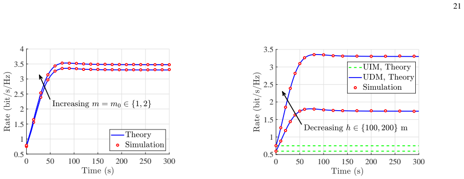
Summary. The paper analyzes a drone cellular network in which drone base stations (DBSs) are initially a homogeneous PPP and then move according to one of four mobility models: straight line (SL), random stop (RS), random walk (RW), or random waypoint (RWP). The serving DBS is chosen by nearest-neighbor association, and two service models are considered (UE independent, UIM, and UE dependent, UDM). The authors derive the temporal point process density of the interfering DBSs via the displacement theorem, provide distributional results for the net displacement under RW and RWP, and express the average received rate and session rate in terms of the conditional Laplace transform of interference. The central comparative claim is Theorem 1: among all i.i.d. mobility models, SL maximizes the expected number of interferers in the disc B = b(o', u0 + vt), and Remark 5 concludes that SL therefore provides a lower bound on the average received rate. Numerical simulations illustrate the ordering of the models.

Significance. If the comparative claim were fully proved, the paper would make a useful contribution: the SL model, which is already used in 3GPP-style simulations, would provide a conservative performance lower bound for a large class of i.i.d. drone mobility models, including curved trajectories. The unified displacement-theorem framework and the explicit density in Lemma 2 are attractive, and the RW/RWP displacement analysis is a genuine technical effort. However, the central comparative theorem is the advertised main novelty, and its proof in Appendix B is not a valid variational argument. The additional step from an expected-count comparison to a rate comparison is also unproved. The paper also overstates exactness by relying on numerical approximations in the RW/RWP rate evaluation. These issues are load-bearing rather than cosmetic, so the contribution in its current form is not ready for publication.

major comments (5)

[Appendix B, Theorem 1, Eq. (27)] The variational proof of Theorem 1 is invalid as written. The integrand in (27) is of the form ux[-g(vt,ux) + FL(u0-ux) + ∫ fL(l)g(l,ux) dl], which is not a functional of the classical form ∫ F(ux, FL(ux), fL(ux)) dux because the dependence on FL is through FL(u0-ux) and the dependence on fL is through an integral of fL(l)g(l,ux) over l. Consequently, the Euler-Lagrange derivatives ∂L/∂FL and d/dux(∂L/∂fL) computed in Appendix B are not standard functional derivatives, and the resulting stationarity condition contains neither FL nor fL. Showing that the integrand vanishes at the two endpoints ux = u0 ± vt does not imply that the integral in (27) is nonnegative for every admissible cdf. Thus Theorem 1 is not established.
[Appendix B, t > u0/v case] The proof of Theorem 1 explicitly handles only t ≤ u0/v and states that t > u0/v 'follows on similar lines'. This is not sufficient because the density in Lemma 2 is structurally different in that regime: the inner region 0 ≤ ux ≤ |u0 - vt| has a nonzero density of λ0 when t > u0/v, whereas it is zero when t ≤ u0/v. A separate argument is needed for the latter case, and the present paper provides none.
[Remark 5, Theorem 1 to average-rate bound] Even if Theorem 1 were true, the conclusion in Remark 5 that 'the average received rate at the typical UE under the SL mobility model is lower compared to the other i.i.d. mobility models' does not follow. The SIR is a nonlinear functional of the entire interfering point process, and the conditional Laplace transform in (22) depends on ux λ(t;ux,u0)(1 - (1 + s(ux^2+h^2)^(-α/2)/m)^(-m)) integrated over all ux. A comparison of the expected number of points in a single fixed disc B = b(o',u0+vt) does not determine this functional. A pointwise domination of the density, or an ordering of the entire interference distribution, would be needed; neither is proved.
[Appendix A, proof of Lemma 2] The proof of Lemma 2, which underpins all subsequent density expressions and Theorem 1, is incomplete. After Eq. (26) the text states that 'simplifying the last step requires tedious integrations and the details are skipped to maintain brevity'. The jump from (26) to the closed-form density in (4)-(5) is a nontrivial derivation and needs to be shown in full, especially because the result is used throughout the paper as the exact point process density.
[Section IV, Remark 6 and Lemma 6] The paper describes its results as 'exact mathematical expressions' for the average and session rates, but the RW and RWP rate expressions depend on two approximations: Remark 6 assumes that Sn and Zn are independent for n ≥ 3, and Lemma 6 provides an approximate pdf for the sum of Rayleigh random variables with constants a0, a1, a2 obtained by numerical curve fitting. The paper should clearly distinguish exact results from approximations and should not claim exactness for metrics that use these fitted and independence-based approximations.

minor comments (5)

[Section VI, Fig. 4 caption] The caption says 'for t ∈ {50, 100, 300} m' but the text states t ∈ {50, 100, 300} s; the units are inconsistent and should be corrected.
[Appendix F, proof of Proposition 2] The proof states that Φn has a 'symmetric triangular distribution' and then immediately concludes Φn ∼ [0,2π). Since Θn and Ψn-1 are independent uniform random variables, the wrapped difference is uniform, not triangular; the intermediate sentence is confusing and should be removed or corrected.
[Section II-C and Eq. (22)] The Nakagami parameter for interferers is defined as mx in the text, but Eq. (22) and the surrounding derivation use a single symbol m; the notation should be made consistent.
[Section II-D] The session rate uses the symbol T for the session duration, while in the RWP model T (or Ti) denotes random waiting times; this notational collision should be avoided for clarity.
[Remark 6] The statement that n ≥ 3 is 'large enough' for the independence approximation to be 'reasonably accurate' is not quantified. A numerical comparison or an error bound should be provided.

Circularity Check

0 steps flagged · score 0.0 of 10

No significant circularity: the paper's derivations are self-contained from the stated PPP and displacement-theorem assumptions, and the self-citations are not load-bearing.

full rationale

I walked the paper's derivation chain from the displacement theorem to the density characterizations in Lemma 2 and Corollary 1, then to the rate expressions in Theorem 2, and finally to the comparative claim in Theorem 1. None of these steps defines one target quantity in terms of itself, fits a parameter to the predicted output, or relies on a self-citation to carry the argument. The SL, RS, RW, and RWP densities are all derived from explicit displacement distributions and the displacement theorem; the rate formula is a standard Laplace-transform/PPP calculation. Theorem 1 compares the intensity measures derived in the same framework, not a quantity fitted from data. The numerical constants in Lemma 6 are auxiliary curve-fitting approximations for Rayleigh sums used in simulations, not inputs to the proof of Theorem 1 or to the rate lower-bound statement. The only self-citations are references [1] and [2], which are the authors' conference versions of this same work; they are mentioned in the footnote but are not cited as evidence for any theorem, uniqueness claim, or modeling ansatz. The variational argument in Appendix B may be mathematically questionable—the Euler-Lagrange computation does not characterize an extremal of the functional, and the proof explicitly defers the t > u0/v case with 'follows on the similar lines'—but this is a correctness or rigor concern, not a circularity. The paper does not reduce its prediction to its inputs by construction; the claimed SL lower bound is an independent, if possibly unsupported, mathematical assertion. I therefore find no circular step under the requested taxonomy and assign score 0.

Assumptions & free parameters 1 free parameters · 5 assumptions · 0 invented entities

The framework relies on standard stochastic geometry and the stated system model. RW and RWP numerical results additionally rely on Rayleigh flights, an unproven independence approximation, and a curve-fitted distribution. The variational proof of Theorem 1 rests on an unproven boundary-extremum premise. No invented physical entities are introduced.

free parameters (1)

a0, a1, a2 in Rayleigh-sum approximation = not reported
In Eq. (10), these constants are obtained by nonlinear curve fitting; values are not given, so reproduction needs to re-run the fit.

assumptions (5)

standard math Displacement theorem for Poisson point processes
Used in Lemma 1 and Lemma 2 to conclude independently displaced points form an inhomogeneous PPP with densities (3)-(6).
domain assumption System assumptions: initial DBSs form a homogeneous PPP, UEs an independent PPP, nearest-neighbor association, constant height, equal powers, Nakagami-m fading
Section II system model, on which all rate expressions rest.
ad hoc to paper Flight distances in RW and RWP are i.i.d. Rayleigh for closed-form displacement results
Lemma 4 uses Rayleigh flights; all plots and rate numbers use Rayleigh flights with mean 500 m. This is a tractability choice, not a physical constraint.
ad hoc to paper Sn and Zn are independent for n >= 3 (Remark 6)
Used to simplify Proposition 1; stated as reasonably accurate without error bounds. All RW and RWP numerical results depend on it.
ad hoc to paper Euler-Lagrange boundary-extremum premise in Appendix B
The proof of Theorem 1 assumes the functional's minimum occurs at the endpoints; this is not generally true and is not proven.

how reviews work

0 comments

Cite this review

Pith. "Pith review of Performance Characterization of Canonical Mobility Models in Drone Cellular Networks." pith.science (2026). https://pith.science/paper/OVVC6AS6

@misc{pith2026190805243,
  author       = {Pith},
  title        = {Pith review of: Performance Characterization of Canonical Mobility Models in Drone Cellular Networks},
  year         = {2026},
  howpublished = {\url{https://pith.science/paper/OVVC6AS6}},
  note         = {Machine review of arXiv:1908.05243}
}

read the original abstract

In this paper, we characterize the performance of several canonical mobility models in a drone cellular network in which drone base stations (DBSs) serve user equipments (UEs) on the ground. In particular, we consider the following four mobility models: (i) straight line (SL), (ii) random stop (RS), (iii) random walk (RW), and (iv) random waypoint (RWP), among which the SL mobility model is inspired by the simulation models used by the third generation partnership project (3GPP) for the placement and trajectory of drones, while the other three are well-known canonical models (or their variants) that offer a useful balance between realism and tractability. Assuming the nearest-neighbor association policy, we consider two service models for the UEs: (i) UE independent model (UIM), and (ii) UE dependent model (UDM). While the serving DBS follows the same mobility model as the other DBSs in the UIM, it is assumed to fly towards the UE of interest in the UDM and hover above its location after reaching there. The main contribution of this paper is a unified approach to characterize the point process of DBSs for all the mobility and service models. Using this, we provide exact mathematical expressions for the average received rate and the session rate as seen by the typical UE. Further, using tools from calculus of variations, we concretely demonstrate that the simple SL mobility model provides a lower bound on the performance of other general mobility models (including the ones in which drones follow curved trajectories) as long as the movement of each drone in these models is independent and identically distributed (i.i.d.). To the best of our knowledge, this is the first work that provides a rigorous analysis of key canonical mobility models for an infinite drone cellular network and establishes useful connections between them.

Figures

Figures reproduced from arXiv: 1908.05243 by the authors.

**Figure 1.** An illustration of the system model. model is already considered sufficient to capture key effects of drone mobility on the systemlevel performance. One can of course generalize this straight-line mobility model to arrive at classical canonical models, such as RW and RWP, which offer a useful balance between realism and tractability. Since all these models are important in their own right, we will develop a unified… view at source ↗

**Figure 2.** Network density in different regions for the SL mobility model. Green and black stars, red circles, and black squares [PITH_FULL_IMAGE:figures/full_fig_p011_2.png] view at source ↗

**Figure 3.** A realization of the RW mobility model. with cdf and pdf of FR(.) and fR(.), respectively [PITH_FULL_IMAGE:figures/full_fig_p013_3.png] view at source ↗

Figures from the paper (6 more)

**Figure 4.** Figure 4: Distribution of L(t) in the RW and RWP mobility models for t ∈ {50, 100, 300} m. As t increases, the pdf of L(t) in both the RW and RWP models converge to a Rayleigh distribution. mobility models, we assume that the flight distances are distributed as i.i.d. Rayleigh r…

**Figure 5.** Figure 5: Density of the network of interfering DBSs for the UDM with the SL and RS mobility models. Serving distance is [PITH_FULL_IMAGE:figures/full_fig_p020_5.png]

**Figure 6.** Figure 6: Density of the network of interfering DBSs for the UDM with the RW and RWP mobility models. Serving distance is [PITH_FULL_IMAGE:figures/full_fig_p020_6.png]

**Figure 7.** Figure 7: Comparison of the average rate for the UDM in the [PITH_FULL_IMAGE:figures/full_fig_p021_7.png]

**Figure 9.** Figure 9: Comparison of the average rate for the UDM in [PITH_FULL_IMAGE:figures/full_fig_p021_9.png]

**Figure 11.** Figure 11: An illustration for the proof of Lemma 2. The red circle and the green dotted circles indicate [PITH_FULL_IMAGE:figures/full_fig_p023_11.png]

Discussion (0). Continue with ORCID to comment.

Reference graph

Works this paper leans on

38 extracted references · 30 canonical work pages

[1]

3GPP-inspired stochastic geometry-based mobility model for a drone cellular network,

M. Banagar and H. S. Dhillon, “3GPP-inspired stochastic geometry-based mobility model for a drone cellular network,” in IEEE Global Commun. Conf. (Globecom) , Dec. 2019

work page 2019
[2]

Fundamentals of drone cellular network analysis under random waypoint mobility model,

——, “Fundamentals of drone cellular network analysis under random waypoint mobility model,” in IEEE Global Commun. Conf. (Globecom), Dec. 2019

work page 2019
[3]

Wireless communications with unmanned aerial vehicles: Opportunities and challenges,

Y . Zeng, R. Zhang, and T. J. Lim, “Wireless communications with unmanned aerial vehicles: Opportunities and challenges,” IEEE Commun. Mag. , vol. 54, no. 5, pp. 36–42, May 2016

2016
[4]

Mobility increases the capacity of ad hoc wireless networks,

M. Grossglauser and D. N. C. Tse, “Mobility increases the capacity of ad hoc wireless networks,” IEEE/ACM Trans. Netw., vol. 10, no. 4, pp. 477–486, Aug. 2002

2002
[5]

The node distribution of the random waypoint mobility model for wireless ad hoc networks,

C. Bettstetter, G. Resta, and P. Santi, “The node distribution of the random waypoint mobility model for wireless ad hoc networks,” IEEE Trans. Mobile Comput. , vol. 2, no. 3, pp. 257–269, July 2003

2003
[6]

Towards understanding the fundamentals of mobility in cellular networks,

X. Lin, R. K. Ganti, P. J. Fleming, and J. G. Andrews, “Towards understanding the fundamentals of mobility in cellular networks,” IEEE Trans. Wireless Commun. , vol. 12, no. 4, pp. 1686–1698, Apr. 2013

2013
[7]

A tutorial on UA Vs for wireless networks: Applications, challenges, and open problems,

M. Mozaffari, W. Saad, M. Bennis, Y . Nam, and M. Debbah, “A tutorial on UA Vs for wireless networks: Applications, challenges, and open problems,” IEEE Commun. Surveys Tut. , to appear
[8]

Enhanced LTE support for aerial vehicles,

3GPP, “Enhanced LTE support for aerial vehicles,” 3rd Generation Partnership Project (3GPP), Tech. Rep. 36.777, 01 2018, version 1.1.0

2018

Show all 38 references

[9]

Enhancement for unmanned aerial vehicles,

——, “Enhancement for unmanned aerial vehicles,” 3rd Generation Partnership Project (3GPP), Tech. Rep. 22.829, 11 2018, version 0.0.0

2018
[10]

Downlink coverage analysis for a ﬁnite 3-D wireless network of unmanned aerial vehicles,

V . V . Chetlur and H. S. Dhillon, “Downlink coverage analysis for a ﬁnite 3-D wireless network of unmanned aerial vehicles,” IEEE Trans. Commun. , vol. 65, no. 10, pp. 4543–4558, Oct. 2017

2017
[11]

Downlink coverage probability in a ﬁnite network of unmanned aerial vehicle (UA V) base stations,

——, “Downlink coverage probability in a ﬁnite network of unmanned aerial vehicle (UA V) base stations,” in IEEE 17th Int. Workshop on Signal Processing Advances in Wireless Commun. , July 2016, pp. 1–5

2016
[12]

Spectrum sharing for drone networks,

C. Zhang and W. Zhang, “Spectrum sharing for drone networks,” IEEE J. Sel. Areas Commun., vol. 35, no. 1, pp. 136–144, Jan. 2017

2017
[13]

Modeling and analysis of aerial base station-assisted cellular networks in ﬁnite areas under LoS and NLoS propagation,

X. Wang, H. Zhang, Y . Tian, and V . C. M. Leung, “Modeling and analysis of aerial base station-assisted cellular networks in ﬁnite areas under LoS and NLoS propagation,” IEEE Trans. Wireless Commun. , vol. 17, no. 10, pp. 6985–7000, Oct. 2018

2018
[14]

Coverage and rate analysis for unmanned aerial vehicle base stations with LoS/NLoS propagation,

M. Alzenad and H. Yanikomeroglu, “Coverage and rate analysis for unmanned aerial vehicle base stations with LoS/NLoS propagation,” in IEEE Global Commun. Conf. Workshops (Globecom Workshops) , Dec. 2018, pp. 1–7

2018
[15]

Unmanned aerial vehicle with underlaid device-to-device communi- cations: Performance and tradeoffs,

M. Mozaffari, W. Saad, M. Bennis, and M. Debbah, “Unmanned aerial vehicle with underlaid device-to-device communi- cations: Performance and tradeoffs,” IEEE Trans. Wireless Commun. , vol. 15, no. 6, pp. 3949–3963, June 2016

2016
[16]

Performance analysis of UA V enabled disaster recovery networks: A stochastic geometric framework based on cluster processes,

A. M. Hayajneh, S. A. R. Zaidi, D. C. McLernon, M. Di Renzo, and M. Ghogho, “Performance analysis of UA V enabled disaster recovery networks: A stochastic geometric framework based on cluster processes,” IEEE Access , vol. 6, pp. 26 215–26 230, 2018. 30

2018
[17]

Fundamentals of modeling ﬁnite wireless networks using binomial point process,

M. Afshang and H. S. Dhillon, “Fundamentals of modeling ﬁnite wireless networks using binomial point process,” IEEE Trans. Wireless Commun., vol. 16, no. 5, pp. 3355–3370, May 2017

2017
[18]

Optimal LAP altitude for maximum coverage,

A. Al-Hourani, S. Kandeepan, and S. Lardner, “Optimal LAP altitude for maximum coverage,” IEEE Wireless Commun. Lett., vol. 3, no. 6, pp. 569–572, Dec. 2014

2014
[19]

A survey of mobility models for ad hoc network research,

T. Camp, J. Boleng, and V . Davies, “A survey of mobility models for ad hoc network research,” Wireless Commun. and Mobile Comput., vol. 2, no. 5, pp. 483–502, 2002

2002
[20]

A survey of mobility models in wireless adhoc networks,

F. Bai and A. Helmy, “A survey of mobility models in wireless adhoc networks,” in Wireless Ad Hoc and Sensor Networks, 2004, pp. 1–30

2004
[21]

Interference and outage in mobile random networks: Expectation, distribution, and correlation,

Z. Gong and M. Haenggi, “Interference and outage in mobile random networks: Expectation, distribution, and correlation,” IEEE Trans. Mobile Comput. , vol. 13, no. 2, pp. 337–349, Feb. 2014

2014
[22]

Fundamentals of mobility-aware performance characterization of cellular networks: A tutorial,

H. Tabassum, M. Salehi, and E. Hossain, “Fundamentals of mobility-aware performance characterization of cellular networks: A tutorial,” IEEE Commun. Surveys Tut. , to appear
[23]

Capacity and delay tradeoffs for ad hoc mobile networks,

M. J. Neely and E. Modiano, “Capacity and delay tradeoffs for ad hoc mobile networks,” IEEE Trans. Inf. Theory, vol. 51, no. 6, pp. 1917–1937, June 2005

1917
[24]

On the latency for information dissemination in mobile wireless networks,

Z. Kong and E. M. Yeh, “On the latency for information dissemination in mobile wireless networks,” in Proc. of the 9th ACM Int. Symp. on Mobile Ad Hoc Netw. and Comput. , May 2008, pp. 139–148

2008
[25]

Shared rate process for mobile users in Poisson networks and applications,

P. Madadi, F. Baccelli, and G. de Veciana, “Shared rate process for mobile users in Poisson networks and applications,” IEEE Trans. Inf. Theory , vol. 64, no. 3, pp. 2121–2141, Mar. 2018

2018
[26]

Stationary distributions of random walk mobility models for wireless ad hoc networks,

M. McGuire, “Stationary distributions of random walk mobility models for wireless ad hoc networks,” in Proc. of the 6th ACM Int. Symp. on Mobile Ad Hoc Netw. and Comput. ACM, 2005, pp. 90–98

2005
[27]

Relaying in mobile ad hoc networks: The Brownian motion mobility model,

R. Groenevelt, E. Altman, and P. Nain, “Relaying in mobile ad hoc networks: The Brownian motion mobility model,” Wireless Netw., vol. 12, no. 5, pp. 561–571, Sep. 2006

2006
[28]

On the Levy-walk nature of human mobility,

I. Rhee et al., “On the Levy-walk nature of human mobility,” IEEE/ACM Trans. Netw., vol. 19, no. 3, pp. 630–643, June 2011

2011
[29]

D. B. Johnson and D. A. Maltz, Dynamic Source Routing in Ad Hoc Wireless Networks . Springer US, 1996, pp. 153–181

1996
[30]

Stochastic properties of the random waypoint mobility model,

C. Bettstetter, H. Hartenstein, and X. Perez-Costa, “Stochastic properties of the random waypoint mobility model,” Wireless Netw., vol. 10, no. 5, pp. 555–567, Sep. 2004

2004
[31]

Spatial node distribution of the random waypoint mobility model with applications,

E. Hyytia, P. Lassila, and J. Virtamo, “Spatial node distribution of the random waypoint mobility model with applications,” IEEE Trans. Mobile Comput. , vol. 5, no. 6, pp. 680–694, June 2006

2006
[32]

Moving aerial base station networks: A stochastic geometry analysis and design perspective,

S. Enayati, H. Saeedi, H. Pishro-Nik, and H. Yanikomeroglu, “Moving aerial base station networks: A stochastic geometry analysis and design perspective,” IEEE Trans. Wireless Commun. , vol. 18, no. 6, pp. 2977–2988, June 2019

2019
[33]

Coverage probability of 3-D mobile UA V networks,

P. K. Sharma and D. I. Kim, “Coverage probability of 3-D mobile UA V networks,” IEEE Wireless Commun. Lett. , vol. 8, no. 1, pp. 97–100, Feb. 2019

2019
[34]

Random 3D mobile UA V networks: Mobility modeling and coverage probability,

——, “Random 3D mobile UA V networks: Mobility modeling and coverage probability,” IEEE Trans. Wireless Commun., vol. 18, no. 5, pp. 2527–2538, May 2019

2019
[35]

Haenggi, Stochastic Geometry for Wireless Networks

M. Haenggi, Stochastic Geometry for Wireless Networks . Cambridge University Press, 2012

2012
[36]

A review of results on sums of random variables,

S. Nadarajah, “A review of results on sums of random variables,” Acta Applicandae Mathematicae , vol. 103, no. 2, pp. 131–140, Sep. 2008

2008
[37]

Accurate simple closed-form approximations to Rayleigh sum distributions and densities,

J. Hu and N. C. Beaulieu, “Accurate simple closed-form approximations to Rayleigh sum distributions and densities,” IEEE Communications Letters , vol. 9, no. 2, pp. 109–111, Feb. 2005

2005
[38]

An interior trust region approach for nonlinear minimization subject to bounds,

T. Coleman and Y . Li, “An interior trust region approach for nonlinear minimization subject to bounds,” SIAM Journal on Optimization, vol. 6, no. 2, pp. 418–445, May 1996

1996

Pith tools

Reviewed August 14, 2026 · model on record in the stance chip above.

[1] [1]

3GPP-inspired stochastic geometry-based mobility model for a drone cellular network,

M. Banagar and H. S. Dhillon, “3GPP-inspired stochastic geometry-based mobility model for a drone cellular network,” in IEEE Global Commun. Conf. (Globecom) , Dec. 2019

work page 2019

[2] [2]

Fundamentals of drone cellular network analysis under random waypoint mobility model,

——, “Fundamentals of drone cellular network analysis under random waypoint mobility model,” in IEEE Global Commun. Conf. (Globecom), Dec. 2019

work page 2019

[3] [3]

Wireless communications with unmanned aerial vehicles: Opportunities and challenges,

Y . Zeng, R. Zhang, and T. J. Lim, “Wireless communications with unmanned aerial vehicles: Opportunities and challenges,” IEEE Commun. Mag. , vol. 54, no. 5, pp. 36–42, May 2016

2016

[4] [4]

Mobility increases the capacity of ad hoc wireless networks,

M. Grossglauser and D. N. C. Tse, “Mobility increases the capacity of ad hoc wireless networks,” IEEE/ACM Trans. Netw., vol. 10, no. 4, pp. 477–486, Aug. 2002

2002

[5] [5]

The node distribution of the random waypoint mobility model for wireless ad hoc networks,

C. Bettstetter, G. Resta, and P. Santi, “The node distribution of the random waypoint mobility model for wireless ad hoc networks,” IEEE Trans. Mobile Comput. , vol. 2, no. 3, pp. 257–269, July 2003

2003

[6] [6]

Towards understanding the fundamentals of mobility in cellular networks,

X. Lin, R. K. Ganti, P. J. Fleming, and J. G. Andrews, “Towards understanding the fundamentals of mobility in cellular networks,” IEEE Trans. Wireless Commun. , vol. 12, no. 4, pp. 1686–1698, Apr. 2013

2013

[7] [7]

A tutorial on UA Vs for wireless networks: Applications, challenges, and open problems,

M. Mozaffari, W. Saad, M. Bennis, Y . Nam, and M. Debbah, “A tutorial on UA Vs for wireless networks: Applications, challenges, and open problems,” IEEE Commun. Surveys Tut. , to appear

[8] [8]

Enhanced LTE support for aerial vehicles,

3GPP, “Enhanced LTE support for aerial vehicles,” 3rd Generation Partnership Project (3GPP), Tech. Rep. 36.777, 01 2018, version 1.1.0

2018