Volterra-series approach to stochastic nonlinear dynamics: linear response of the Van der Pol oscillator driven by white noise

A.J. Hudspeth; Florian Berger; Roman Belousov

REVIEW 3 major objections 5 minor 49 references

Volterra-series approach to stochastic nonlinear dynamics: linear response of the Van der Pol oscillator driven by white noise

T0 review · 3 major / 5 minor · reviewed 2026-08-14 · deepseek-v4-flash

Challenge this review Re-run · record.json Download PDF Read on arXiv ↗ Review JSON

Pith's one-line read A white-noise-driven Van der Pol oscillator can be treated, to first order in the noise, as a single-mode relaxation cycle plus a Gaussian linear-response term, yielding explicit statistics and a parameter-inference method.

desk verdict A practical Volterra-based parameter-inference method for noisy Van der Pol oscillators, credible for moderate noise but with an uncontrolled period-averaging step that deserves scrutiny. read the letter →

arxiv 1908.05313 v2 pith:WEXROISE submitted 2019-08-14 cond-mat.stat-mech nlin.CD

Roman Belousov , Florian Berger , A.J. Hudspeth This is my paper · ORCID

classification cond-mat.stat-mechnlin.CD MSC 34C1534F0560H10 PACS 05.40.-a05.45.-a02.50.Ey

keywords VanderPoloscillatorwhitenoiseVolterraserieslinearresponserelaxationoscillationsparameterinferencehairbundleautocorrelationfunction

verification ladder T0 review T1 audit T2 compute T3 formal

The pith

A machine-rendered reading of the paper's core claim, the machinery that carries it, and where it could break.

The reading

This paper claims that the Van der Pol oscillator driven by white noise can be understood, to first order in the noise, as a deterministic relaxation cycle plus an independent Gaussian linear-response term. The deterministic part is approximated by a single harmonic mode, and the noise response by a damped harmonic oscillator whose friction and stiffness are the period-averaged coefficients of the linearized equation. From that decomposition the authors derive closed-form expressions for the autocorrelation function, variance, and characteristic function, and turn them into a two-step parameter-estimation procedure. If the approximation holds, a researcher can extract the oscillator's friction, stiffness, and damping parameters directly from a measured noisy time series, and can build a linear surrogate model that mimics the underlying nonlinear oscillator.

What carries the argument

The load-bearing object is the first-order Volterra kernel $g_\xi(t)=\Omega^{-1}\exp(-\langle a_\xi\rangle t/2)\sin(\Omega t)$, the linear response of the period-averaged variational equation. The variational equation around the limit cycle has time-periodic coefficients; replacing them by their period averages turns the response into that of a constant-coefficient harmonic oscillator, so the noise-driven part becomes Gaussian with a known autocovariance. The single-mode approximation $\xi_0(t)=\alpha\cos(\sqrt{b}\,t)$ with $\alpha=2\sqrt{-a/c}$ supplies the deterministic part and makes the averaging and the statistics explicit, including the arcsine law for the autonomous term and a Bessel-function characteristic function for the sum.

What would settle it

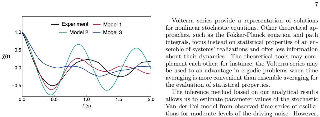
Simulate Eq. (1) with $\mu=2$ and $A=0.6$, then compare the empirical autocorrelation function against the theoretical expression of Eq. (B8); if the discrepancy exceeds the claimed 15% parameter error, the single-mode period-averaging assumption fails. Alternatively, measure the empirical linear response to a weak probe force and check whether it matches the kernel $g_\xi(t)$ of Eq. (12).

Watch

Extended reading notes

Core claim

The central discovery is that the stochastic Van der Pol solution admits the approximate representation $x(t)\approx \xi(t)+\int_0^t g_\xi(t-s)f(s)\,ds$, in which $\xi(t)=\alpha\cos(\sqrt{b}\,t)$ is the single-mode limit cycle and $g_\xi$ is the Green function of a damped harmonic oscillator with effective coefficients $\langle a_\xi\rangle$ and $\langle b_\xi\rangle$ obtained by averaging the time-dependent linearized coefficients over one period. This reduces a nonlinear relaxation oscillator to a linear system driven by the same noise, and yields explicit formulas for the autocorrelation function and variance. The paper also claims that fitting measured autocorrelations and oscillatory trends to these formulas recovers $a$, $b$, $c$, and the noise amplitude $A$ within about 15% for moderate noise ($0.2<A<1.2$ at $\mu=1$), with $b$ the most biased parameter and $\mu$ within 10%.

Load-bearing premise

That the Van der Pol limit cycle can be represented by the single harmonic $\xi(t)=\alpha\cos(\sqrt{b}\,t)$ and that the time-dependent linearized coefficients can be replaced by their period averages, an approximation the paper verifies only by simulation for $\mu=1$ and moderate noise, without a rigorous error bound.

Editorial extensions

If this is right

Any measured time series whose autocorrelation matches the derived expression over its early decay can be mapped to Van der Pol parameters without solving the nonlinear equation numerically.
The decomposition provides a linear surrogate: a driven harmonic oscillator plus periodic forcing reproduces the statistics of the nonlinear relaxation oscillations, which is useful for engineering and biological modeling.
The inference method cannot resolve very small noise amplitudes because the deterministic trend dominates, and its precision deteriorates as the nonlinearity parameter $\mu$ grows.
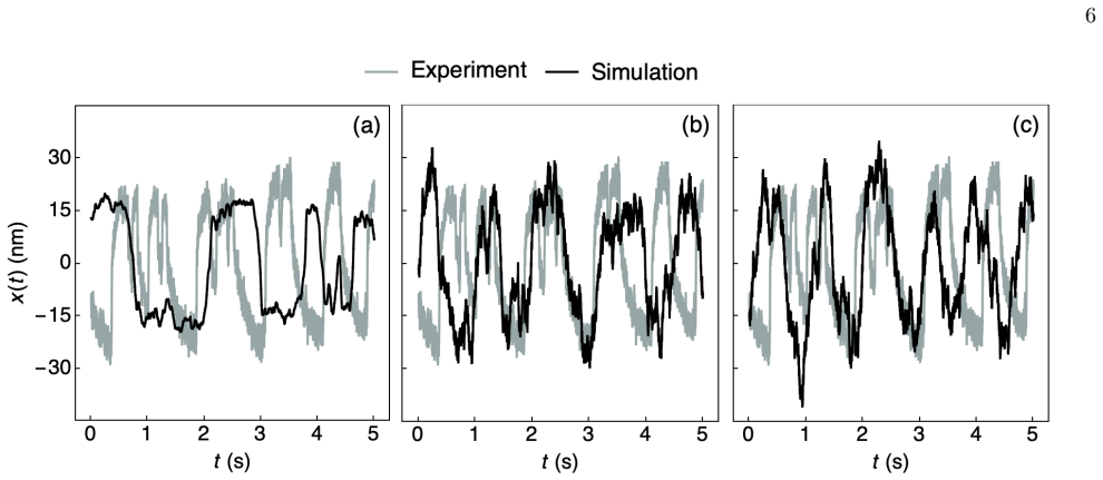
For hair-bundle oscillations, the simple Van der Pol equation is rejected by the data, while a hidden Van der Pol oscillator linearly coupled to the measured coordinate reproduces the observations, with an effective linear model nearly indistinguishable from it.

Reading between the lines

Editorial extensions of the paper, not claims the author makes directly.

The same period-averaging trick should extend to other Lienard-class oscillators, but the single-mode approximation will break down as the limit cycle develops strong harmonics; the paper's own $\mu>1$ caveat suggests a quantitative boundary worth testing.
The phase-diffusion effect the paper identifies, noise-induced shifts near the origin of phase space, implies that the autocorrelation formulas are trustworthy only on time scales short compared with phase decorrelation; a polar-coordinate treatment would likely replace the persistent cosine term by an exponentially decaying envelope.
One could turn the linear surrogate into a generative model for synthetic data, simulating the effective driven oscillator with fitted parameters and using it for detector design or hypothesis testing in sensory neuroscience.
A direct experimental test would be to apply a weak sinusoidal probe force and measure the empirical linear response function; if it matches $g_\xi(t)$ within the stated noise range, the core approximation is confirmed directly rather than through autocorrelation fits.

Share X Bluesky LinkedIn Reddit HN

Signed reviews

No signed human review yet.

Editorial analysis

A structured set of objections, weighed in public.

Desk editor's note, referee report, and a circularity audit.

Desk Editor's Note

read the letter

Here's the short version: this is a useful methods paper that extends the Volterra linear-response approach from the Duffing oscillator to the Van der Pol oscillator, and the proposed inference recipe appears to work at the 10-15% level for moderate noise. The main weakness is that the period-averaging step that turns the linearized equation into a constant-coefficient damped oscillator is not controlled. The exact linearization about a limit cycle has a zero Floquet mode, so the averaged kernel is missing a non-decaying component. The paper knows this—it discusses phase diffusion and restricts the autocorrelation fit to short times—but it never shows how much error that introduces. The sign typo in Eq. (11) (should be +⟨aξ⟩ times the velocity) and the one in Eq. (18) (the square root needs −ab, not ab) are minor but should be fixed.

What's genuinely new is the Van der Pol extension itself. Unlike Duffing, the limit cycle has no closed form, the stationary density is singular, and phase diffusion is a real effect. The single-mode approximation plus period averaging is a pragmatic choice, and Table I shows the inference method works for moderate noise. The hidden Van der Pol model for hair-bundle oscillations is a nice demonstration that the approach can adapt to real data. The paper is also honest about its limits: it explicitly says the method degrades for small and large noise, and that phase fluctuations are the major challenge.

The big soft spot is the period averaging. The stress-test note is correct: the linear response of the true system contains a term proportional to the derivative of the limit cycle, which does not decay, while the averaged kernel has artificial damping. The paper's defense is that only short-time behavior is used, but it doesn't quantify the effect on the fit. Table I is a simulation check, which is useful, but it doesn't isolate this particular error. A referee could reasonably ask for a numerical comparison with the full Floquet response in a few parameter regimes. Also, the fitting procedure relies on nuisance parameters λ1 and λ2 in Eq. (15) that are fitted rather than predicted—acceptable for a practical tool, but it reduces inferential power.

The experimental section is qualitative: the simple Van der Pol model clearly fails, the hidden Van der Pol matches, but there is no quantitative goodness-of-fit measure. That's fine for a demonstration, but not a strong validation.

If I were editing, I'd send this to peer review. The central approximation is reasonable, the method is practical, and the paper is honest about its shortcomings. A referee should ask for a discussion of the zero-Floquet-mode issue (and preferably a numerical check), plus the typo fixes. For a reader working on stochastic oscillators or hair-cell biophysics, this is worth reading and citing. It doesn't reorganize the field, but it gives a workable tool.

Referee Report

3 major / 5 minor

Summary. The paper develops an approximate analytic treatment of the Van der Pol oscillator driven by white noise. The authors expand the solution in a Volterra series around the limit-cycle solution and approximate the limit cycle by a single harmonic ξ(t) = α cos(√b t) (Eq. A3). Linearizing around ξ(t) gives a time-periodic variational equation (Eq. 6), whose coefficients are then replaced by their period averages (Eqs. 9–11), yielding a damped harmonic oscillator with response kernel g_ξ(t) (Eq. 12) and approximate solution x_ξ(t) = ξ(t) + ∫ g_ξ(t−s) f(s) ds (Eq. 13). From this approximation the paper derives the autocorrelation function (Eqs. B7–B8), the characteristic function (Eq. B4), and a two-step parameter-inference scheme: fit the autocorrelation to obtain a and b, then fit half-period trajectory pieces to obtain c and A (Eqs. 15–18). The method is tested on simulations (Table I) and applied to hair-bundle experimental data, where the simple Van der Pol model fails but a hidden Van der Pol system (Eqs. 20–21) and an effective linear model reproduce the data.

Significance. Should the approximation hold, the paper offers a simple and broadly useful route: a nonlinear stochastic oscillator is reduced to a driven damped harmonic oscillator, giving closed-form statistics and a practical inference protocol. The paper's strengths are explicit analytical formulas, validation against simulations for μ = 1 and moderate noise, and an experimental application with a clear negative result for the simple model. The method is not circular: the parameter estimates are calibrated against simulated data with known parameters, and the experimental application is a genuine out-of-sample use. However, the central reduction is heuristic; the main value would be greatly strengthened by a quantitative justification of the period-averaging step and a demonstration of the robustness of the fitting window.

major comments (3)

[II A, Eqs. (6)–(13)] The replacement of the time-periodic coefficients a_ξ(t) and b_ξ(t) by their period averages is the load-bearing step of the paper, but its accuracy is not established. The exact variational equation about a stable limit cycle has a zero Floquet exponent corresponding to phase shifts; the averaged oscillator (11) has two complex exponents with real part −⟨a_ξ⟩/2 < 0. Hence the exact linear response contains a non-decaying component proportional to the derivative of the limit cycle that g_ξ(t) in Eq. (12) cannot represent. For stochastic forcing this discarded mode is responsible for the phase diffusion acknowledged in Sec. II A and Appendix B. The statement that the approximation is valid on short times does not by itself justify the fitting interval 0 ≤ t ≤ τ, because the discarded mode contributes on all time scales. I ask the authors to provide a quantitative comparison with the exact Floquet response of Eq. (6) (for example, by numerically computing its fundamental matrix) and to state the resulting error bounds on the inference formulas.
[Table I and Sec. II B] The claim that the inferred parameter values are accurate within 15% is not supported by an error analysis that propagates the approximations through the fitting procedure. The autocorrelation fit (Eq. 15) depends on two fitted nuisance amplitudes λ1 and λ2, the chosen window τ, and the initial guesses described in Sec. II B, while the amplitude/variance step (Eq. 18) uses the sample variance ⟨x²⟩ whose relation to the theoretical variance is affected by phase diffusion. The paper tests one value μ = 1 and a specific set of noise amplitudes, but it does not quantify how the bias in Table I changes with the fitting window or with μ near the stated range of validity. Adding a sensitivity study of the window length, noise amplitude, and initial guesses, together with fitting residuals, is necessary to support the stated accuracy.
[Appendix A and Sec. II B] The single-mode approximation ξ0(t) for the limit cycle itself is uncontrolled. The authors provide two levels ξ0 and ξ1, but Fig. 4 shows that ξ1 is visibly closer to the simulated limit cycle, while the paper nevertheless uses ξ0 for the variance and amplitude step (Eq. 18) because ξ1 overestimates ⟨x²⟩. This mixed use of the two approximations is not systematically justified. A consistent error estimate for the limit-cycle approximation, for example from the next Picard iterate or from the omitted harmonic, is needed before the inference formulas can be regarded as quantitative.

minor comments (5)

[Eq. (11)] There is a sign typo in Eq. (11): since ⟨a_ξ⟩ ≈ −a > 0, the equation should read +⟨a_ξ⟩ γ̇, not −⟨a_ξ⟩ γ̇, for consistency with the decaying response in Eq. (12).
[Fig. 6 caption] The caption refers to “χ1(t) [Eq. (1)]”; this should be Eq. (B8).
[Throughout] There are several typographical errors: “Comparision” in the Fig. 2 caption, “expeirments” in the Fig. 3 caption, “self-sustatined” in the Conclusion, and a stray “v,” before the coefficient definitions in Appendix D. These should be corrected.
[Eq. (15)] Equation (15) is extremely dense and difficult to parse; splitting it into a prefactor and a bracket, or introducing auxiliary variables for Ω and the µ-dependent damping, would substantially improve readability.
[Reference [43]] Reference [43] is incomplete: it lacks journal, volume, and page information and should be completed.

Circularity Check

0 steps flagged · score 0.0 of 10

No significant circularity: the central approximation is derived in-paper and validated against simulations with known parameters; the fitted nuisance amplitudes do not force the inferred physics.

full rationale

The paper's central object is the linear-response approximation x(t) ≈ ξ(t) + ∫ g_ξ(t−s) f(s) ds, Eq. (13). This is not an input restated as an output: the kernel g_ξ is computed from the period-averaged coefficients ⟨a_ξ⟩ and ⟨b_ξ⟩ of the linearized variational equation, Eqs. (9)–(12), and the limit-cycle approximation ξ(t) is derived in Appendix A by harmonic-balance/variational Green's-function methods, Eqs. (A2)–(A4). The replacement of time-periodic coefficients by their period averages is an uncontrolled approximation, and the paper explicitly admits its limitations, saying the approximate solution is valid only for small noise and that time autocorrelations coincide with simulations only at small t (Sec. II A, Appendix B). That is a correctness or accuracy concern, not circularity: the approximation is checked against direct simulation rather than assumed. The inference method in Sec. II B fits the autocorrelation formula Eq. (15) with explicit nuisance amplitudes λ1 and λ2. The paper states these are 'determined up to an arbitrary factor' and 'treated as nuisance parameters,' so they are fitted degrees of freedom, not predictions; moreover, the parameters of interest a, b, c, and A are validated in Table I against simulated data with known values a = −1, b = 1, c = 1. The derived relations c = −4a/α^2 and A = √[ab(2⟨x²⟩ − α²)] in Eq. (18) are algebraic identities connecting fitted amplitude and variance to the model parameters; because the amplitude is measured from the trajectory and the result is compared with known simulation inputs, no quantity reduces to itself by construction. The experimental section is explicitly a demonstration of how the method can be applied, not a claim that the simplified Van der Pol model predicts the hair-bundle data without fitting; the paper in fact reports that the simple model does not reproduce the data. Self-citations, especially the companion Duffing paper Ref. [23], supply context and numerical/simulation techniques, but the Van der Pol derivation, the autocorrelation formulas, and the validation against simulated data are carried out in the present manuscript. The period-averaging and zero-Floquet-mode issue raised by the skeptical reader is a legitimate approximation risk, but it is not a circular reduction of the paper's conclusions to its inputs. Overall, no circular step meeting the required evidentiary standard was found.

Assumptions & free parameters 2 free parameters · 5 assumptions · 1 invented entities

The central theoretical claim rests on four uncontrolled approximations: truncated Volterra series, single-harmonic limit cycle, period-averaged coefficients, and neglect of phase diffusion. The inference adds fitted nuisance amplitudes. The only invented entity is the hidden vdP coordinate for the biological application, which has no independent evidence beyond fitting the measured coordinate.

free parameters (2)

lambda1 = fitted per time series
Amplitude of the periodic term in the theoretical autocorrelation Eq. (15); treated as a nuisance parameter, so the autocorrelation shape is not parameter-free.
lambda2 = fitted per time series
Amplitude of the decaying term in Eq. (15); treated as a nuisance parameter.

assumptions (5)

domain assumption The Volterra series expansion Eq. (2) converges or is valid as a truncated first-order expansion for the noisy Van der Pol equation at the noise levels considered.
Invoked in Sec. II A; the paper notes the series may fail to exist and is restricted by a radius of convergence, and validates only by simulations.
domain assumption The limit-cycle solution x0(t) is adequately represented by the single-mode Fourier approximation xi0(t) = alpha cos(sqrt(b) t), with frequency sqrt(b) and amplitude 2 sqrt(-a/c).
Used throughout Sec. II and Appendices A-B; corrections are O(mu^2) in frequency and the paper notes Eq. (A4) captures asymmetry better but overestimates variance.
domain assumption Replacing the periodic coefficients a_xi(t) and b_xi(t) by their time averages yields a valid effective harmonic oscillator for the linear response gamma1(t).
Eqs. (9)-(11); no error bound is provided, and the justification is analogy to time-averaging methods plus numerical agreement.
domain assumption Phase fluctuations of the noisy oscillation average to zero and do not affect time-invariant statistics, while autocorrelations are only trusted at small times.
Discussed in Sec. II A and Appendix B; the paper acknowledges this as a major limitation.
domain assumption The parsimonious hair-bundle model of Ref. [37] can be reduced to the hidden Van der Pol system Eqs. (20)-(21) via the overdamped limit M/Gamma to 0 and K2 approximately equal to K3.
Appendix D applies strong simplifications to the published biological model; this assumption affects the experimental demonstration only.

invented entities (1)

Hidden Van der Pol oscillator z(t) in Eqs. (20)-(21)
purpose: Represents an unobserved degree of freedom that, linearly coupled to the measured coordinate x(t), reproduces hair-bundle oscillations.
Derived from the published model of O Maoileidigh et al. [37] by overdamped limit and K2 about K3; no direct experimental observation of z(t) is provided, only an indirect fit to x(t).

how reviews work

0 comments

Cite this review

Pith. "Pith review of Volterra-series approach to stochastic nonlinear dynamics: linear response of the Van der Pol oscillator driven by white noise." pith.science (2026). https://pith.science/paper/WEXROISE

@misc{pith2026190805313,
  author       = {Pith},
  title        = {Pith review of: Volterra-series approach to stochastic nonlinear dynamics: linear response of the Van der Pol oscillator driven by white noise},
  year         = {2026},
  howpublished = {\url{https://pith.science/paper/WEXROISE}},
  note         = {Machine review of arXiv:1908.05313}
}

read the original abstract

The Van der Pol equation is a paradigmatic model of relaxation oscillations. This remarkable nonlinear phenomenon of self-sustained oscillatory motion underlies important rhythmic processes in nature and electrical engineering. Relaxation oscillations in a real system are usually coupled to environmental noise, which further enriches their dynamics, but makes theoretical analysis of such systems and determination of the equation's parameter values a difficult task. In a companion paper we have proposed an analytic approach to a similar problem for another classical nonlinear model, the bistable Duffing oscillator. Here we extend our techniques to the case of the Van der Pol equation driven by white noise. We analyze the statistics of solutions and propose a method to estimate parameter values from the oscillator's time series. We use experimental data of active oscillations in a biological system to demonstrate how our method applies to real observations and how it can be generalized for more complex models.

Figures

Figures reproduced from arXiv: 1908.05313 by the authors.

**Figure 2.** FIG. 2. Comparision of three models for hair-cell bundle oscillations with the experimental data. Panel (a): The simple Van [PITH_FULL_IMAGE:figures/full_fig_p006_2.png] view at source ↗

**Figure 3.** FIG. 3. Comparison of the empirical time autocorrelation [PITH_FULL_IMAGE:figures/full_fig_p007_3.png] view at source ↗

Figures from the paper (3 more)

**Figure 4.** Figure 4: FIG. 4. Comparison of the approximate solution [PITH_FULL_IMAGE:figures/full_fig_p009_4.png]

**Figure 5.** Figure 5: FIG. 5. Comparison of the theoretical expression given by Eq. (B4) with the empirical characteristic function [PITH_FULL_IMAGE:figures/full_fig_p009_5.png]

**Figure 6.** Figure 6: FIG. 6. Comparison of the theoretical expression [PITH_FULL_IMAGE:figures/full_fig_p010_6.png]

Discussion (0). Continue with ORCID to comment.

Reference graph

Works this paper leans on

49 extracted references · 46 canonical work pages

[1]

(1) withf≡ 0

˙γ1 + (b + 2c ˙x0x0)γ1 = f, (5) ··· Equation (4), which uniquely deﬁnes x0(t) for a given initial condition ( x(0), ˙x(0) ) , is equivalent to the au- tonomous Van der Pol problem—Eq. (1) withf≡ 0. The linear Eq. (5), which determines the ﬁrst-order Volterra term γ1(t), in general contains time-dependent coeﬃ- cients. Because the Volterra series generaliz...

work page
[2]

Ginoux and C

J.-M. Ginoux and C. Letellier, Chaos: An Interdisci- plinary Journal of Nonlinear Science 22, 023120 (2012)

work page 2012
[3]

van der Pol, The London, Edinburgh, and Dublin Philosophical Magazine and Journal of Science 2, 978 (1926)

B. van der Pol, The London, Edinburgh, and Dublin Philosophical Magazine and Journal of Science 2, 978 (1926)

work page 1926
[4]

Beta and K

C. Beta and K. Kruse, Annual Review of Condensed Mat- ter Physics 8, 239 (2017)

work page 2017
[5]

S. H. Strogatz, Nonlinear Dynamics and Chaos: With Applications to Physics, Biology, Chemistry, and Engi- neering, 2nd ed. (Avalon Publishing, 2014)

work page 2014
[6]

Buzs´ aki and A

G. Buzs´ aki and A. Draguhn, Science304, 1926 (2004)

work page 2004
[7]

A. C. Oates, L. G. Morelli, and S. Ares, Development 139, 625 (2012)

2012
[8]

Rompala, R

K. Rompala, R. Rand, and H. Howland, Communica- tions in Nonlinear Science and Numerical Simulation 12, 794 (2007)

work page 2007

Show all 49 references

[9]

Nomura, S

T. Nomura, S. Sato, S. Doi, J. P. Segundo, and M. D. Stiber, Biological cybernetics 69, 429 (1993)

1993
[10]

C. L. Talmadge, G. R. Long, W. J. Murphy, and A. Tubis, The Mechanics and Biophysics of Hearing , , 235 (1990)

1990
[11]

Duifhuis, H

H. Duifhuis, H. W. Hoogstraten, S. M. van Netten, R. J. Diependaal, and W. Bialek, Peripheral Auditory Mech- anisms, , 290 (1986)

1986
[12]

van der Pol, The London, Edinburgh, and Dublin Philosophical Magazine and Journal of Science 6, 763 (1928)

B. van der Pol, The London, Edinburgh, and Dublin Philosophical Magazine and Journal of Science 6, 763 (1928)

1928
[13]

van Dijk and H

P. van Dijk and H. P. Wit, The Journal of the Acoustical Society of America 88, 1779 (1990)

1990
[14]

R. E. Mirollo and S. H. Strogatz, SIAM Journal on Ap- plied Mathematics 50, 1645 (1990)

1990
[15]

van der Pol, Acta Medica Scandinavica103, 76 (1940)

B. van der Pol, Acta Medica Scandinavica103, 76 (1940)

1940
[16]

A. A. Cherevko, E. E. Bord, A. K. Khe, V. A. Panarin, and K. J. Orlov, Journal of Physics: Conference Series 894, 012012 (2017)

2017
[17]

A. A. Cherevko, A. V. Mikhaylova, A. P. Chupakhin, I. V. Uﬁmtseva, A. L. Krivoshapkin, and K. Y. Orlov, Journal of Physics: Conference Series 722, 012045 (2016)

2016
[18]

Nagumo, S

J. Nagumo, S. Arimoto, and S. Yoshizawa, Proceedings of the IRE 50, 2061 (1962)

1962
[19]

FitzHugh, Biophysical Journal 1, 445 (1961)

R. FitzHugh, Biophysical Journal 1, 445 (1961)

1961
[20]

Alonso, F

R. Alonso, F. Goller, and G. B. Mindlin, Physical Review E 89 (2014), 10.1103/PhysRevE.89.032706

2014 doi
[21]

Izhikevich and R

E. Izhikevich and R. FitzHugh, Scholarpedia 1, 1349 (2006)

2006
[22]

Roenneberg, E

T. Roenneberg, E. J. Chua, R. Bernardo, and E. Men- doza, Current Biology 18, R826 (2008)

2008
[23]

This approach unfortunately fails in the case of the noisy Van der Pol oscillator: such an expansion may not exist near the two singularities at which p(ξ0) tends to inﬁnity

we have succeeded in ﬁtting a bimodal probability density of the noisy Duﬃng oscillator to an approximate expression that was derived from a power series for the exponential family of random variables. This approach unfortunately fails in the case of the noisy Van der Pol osci...
[24]

G. B. Mindlin, Chaos: An Interdisciplinary Journal of Nonlinear Science 27, 092101 (2017)

2017
[25]

Belousov, F

R. Belousov, F. Berger, and A. J. Hudspeth, Physical Review E 99 (2019), 10.1103/physreve.99.042204

2019 doi
[26]

Schetzen, The Volterra and Wiener Theories of Non- linear Systems (Krieger Pub., 2006)

M. Schetzen, The Volterra and Wiener Theories of Non- linear Systems (Krieger Pub., 2006)

2006
[27]

W. J. Rugh, Nonlinear System Theory: The Volterra/Wiener Approach (Johns Hopkins Univer- sity Press, 1981)

1981
[28]

Jordan and P

D. Jordan and P. Smith, Nonlinear Ordinary Diﬀerential Equations:An Introduction for Scientists and Engineers: An Introduction for Scientists and Engineers (OUP Ox- ford, 2007)

2007
[29]

Grimshaw, Nonlinear ordinary diﬀerential equations (CRC Press, Boca Raton, 2017)

R. Grimshaw, Nonlinear ordinary diﬀerential equations (CRC Press, Boca Raton, 2017)

2017
[30]

Belousov and E

R. Belousov and E. G. D. Cohen, Physical Review E 94 (2016), 10.1103/PhysRevE.94.062124

2016 doi
[31]

Chandrasekhar, Rev

S. Chandrasekhar, Rev. Mod. Phys. 15, 1 (1943)

1943
[32]

A. N. Lagar’kov and V. M. Sergeev, Soviet Physics Us- pekhi 21, 566 (1978)

1978
[33]

A. J. Hudspeth, Nature Reviews Neuroscience 15, 600 (2014)

2014
[34]

Martin and A

P. Martin and A. J. Hudspeth, Proceedings of the Na- tional Academy of Sciences 96, 14306 (1999)

1999
[35]

Faber and D

J. Faber and D. Bozovic, Scientiﬁc Reports 8, 1 (2018)

2018
[36]

Nadrowski, P

B. Nadrowski, P. Martin, and F. J¨ ulicher, Proceedings of the National Academy of Sciences 101, 12195 (2004)

2004
[37]

Tinevez, F

J.-Y. Tinevez, F. J¨ ulicher, and P. Martin, Biophysical Journal 93, 4053 (2007)

2007
[38]

Barral, K

J. Barral, K. Dierkes, B. Lindner, F. Julicher, and P. Martin, Proceedings of the National Academy of Sci- ences 107, 8079 (2010)

2010
[39]

O Maoileidigh, E

D. O Maoileidigh, E. M. Nicola, and A. J. Hudspeth, Proceedings of the National Academy of Sciences 109, 1943 (2012)

2012
[40]

J. B. Azimzadeh and J. D. Salvi, JoVE (Journal of Vi- sualized Experiments) , e55380 (2017)

2017
[41]

J. B. Azimzadeh, B. A. Fabella, N. R. Kastan, and A. J. Hudspeth, Neuron 97, 586 (2018)

2018
[42]

These experiments were conducted in a sample chamber that was cooled down to 285 K by a peltier element and in accordance with the policies of The Rockefeller Uni- versity’s Institutional Animal Care and Use Committee (IACUC Protocol 16942)
[43]

Gelfand, O

M. Gelfand, O. Piro, M. O. Magnasco, and A. J. Hud- speth, PLoS ONE 5, e11116 (2010)

2010
[44]

D. T. Raphael, The Journal of the Acoustical Society of America 94, 428 (1993)

1993
[45]

S. A. Khuri and A. Sayfy, , 9 (2017)

2017
[46]

Abukhaled, Journal of Computational and Nonlinear Dynamics 12, 051021 (2017)

M. Abukhaled, Journal of Computational and Nonlinear Dynamics 12, 051021 (2017)

2017
[47]

Balakrishnan and V

N. Balakrishnan and V. B. Nevzorov, A Primer on Sta- tistical Distributions (John Wiley & Sons, 2004)

2004
[48]

Tuckerman, B

M. Tuckerman, B. J. Berne, and G. J. Martyna, The Journal of Chemical Physics 97, 1990 (1992)

1992
[49]

Belousov, E

R. Belousov, E. G. D. Cohen, and L. Rondoni, Physical Review E 96 (2017), 10.1103/PhysRevE.96.022125

2017 doi

Pith tools

Reviewed August 14, 2026 · model on record in the stance chip above.

[1] [1]

(1) withf≡ 0

˙γ1 + (b + 2c ˙x0x0)γ1 = f, (5) ··· Equation (4), which uniquely deﬁnes x0(t) for a given initial condition ( x(0), ˙x(0) ) , is equivalent to the au- tonomous Van der Pol problem—Eq. (1) withf≡ 0. The linear Eq. (5), which determines the ﬁrst-order Volterra term γ1(t), in general contains time-dependent coeﬃ- cients. Because the Volterra series generaliz...

work page

[2] [2]

Ginoux and C

J.-M. Ginoux and C. Letellier, Chaos: An Interdisci- plinary Journal of Nonlinear Science 22, 023120 (2012)

work page 2012

[3] [3]

van der Pol, The London, Edinburgh, and Dublin Philosophical Magazine and Journal of Science 2, 978 (1926)

B. van der Pol, The London, Edinburgh, and Dublin Philosophical Magazine and Journal of Science 2, 978 (1926)

work page 1926

[4] [4]

Beta and K

C. Beta and K. Kruse, Annual Review of Condensed Mat- ter Physics 8, 239 (2017)

work page 2017

[5] [5]

S. H. Strogatz, Nonlinear Dynamics and Chaos: With Applications to Physics, Biology, Chemistry, and Engi- neering, 2nd ed. (Avalon Publishing, 2014)

work page 2014

[6] [6]

Buzs´ aki and A

G. Buzs´ aki and A. Draguhn, Science304, 1926 (2004)

work page 2004

[7] [7]

A. C. Oates, L. G. Morelli, and S. Ares, Development 139, 625 (2012)

2012

[8] [8]

Rompala, R

K. Rompala, R. Rand, and H. Howland, Communica- tions in Nonlinear Science and Numerical Simulation 12, 794 (2007)

work page 2007