Numerical solution for tachyon vacuum in the Schnabl gauge

E. Aldo Arroyo; Mat\v{e}j Kudrna

REVIEW 4 major objections 6 minor 45 references

Numerical solution for tachyon vacuum in the Schnabl gauge

T0 review · 4 major / 6 minor · reviewed 2026-08-14 · deepseek-v4-flash

Challenge this review Re-run · record.json Download PDF Read on arXiv ↗ Review JSON

Pith's one-line read This paper claims that a level-24 numerical solution in the Schnabl gauge converges to the analytic tachyon vacuum, with extrapolated energy within 0.05 percent of -1.

desk verdict Genuinely reusable numerical method and L=24 Schnabl-gauge data; the infinite-level claims are suggestive, but the extrapolation error bars are not controlled. read the letter →

arxiv 1908.05330 v3 pith:WCYJ3UUF submitted 2019-08-14 hep-th

E. Aldo Arroyo , Matěj Kudrna This is my paper · ORCID

classification hep-th

keywords tachyonvacuumSchnablgaugeleveltruncationopenstringfieldtheorySen'sfirstconjectureEllwoodinvariantNewton'smethodfixing

verification ladder T0 review T1 audit T2 compute T3 formal

The pith

A machine-rendered reading of the paper's core claim, the machinery that carries it, and where it could break.

The reading

This paper tries to establish that the numerical tachyon-vacuum solution obtained by level truncation in the Schnabl gauge becomes the analytic tachyon vacuum as the level goes to infinity. To get there, the authors develop a projector-based Newton method that lets them solve the level-truncated equations of motion up to level 24, far beyond the previous level-10 limit. Their evidence is that the vacuum energy has its predicted local minimum at level 12 and extrapolates to about -0.9995, matching -1 at roughly the 0.05 percent level; the gauge-invariant overlap extrapolates to about -0.0015, within 0.15 percent of zero; and the equations of motion that were projected out during gauge fixing vanish asymptotically. If this identification is right, Sen's first conjecture holds numerically in the Schnabl gauge, with somewhat lower precision than in the Siegel gauge.

What carries the argument

The load-bearing machinery is a canonical projector $P_C$ constructed from the matrix $G$ of the gauge condition $B_0\Psi = 0$. The projector divides string-field coefficients into dependent and independent variables, so Newton's method can solve only the projected equations of motion without ever storing the full cubic vertex; this reduction is what makes level 24 reachable when storing the full vertex would need more than a petabyte. The second piece of machinery is the extrapolation ansatz $q_M^{(L_{\min},L_{\max})}(L) = a_0 + \sum_{n=1}^{M} a_n/L^n$, supplemented by a second fit in $1/N$ of order $M=5$, used to estimate infinite-level values of the energy, the coefficients, and the Ellwood invariant.

What would settle it

Compute the same Schnabl-gauge solution at levels 26, 28, and 30 with the projector-based Newton method and rerun the maximal-order $1/L$ polynomial extrapolations; if the predicted infinite-level energy moves away from $-1$ by more than the stated $10^{-4}$ error, or if the coefficients stop tracking the analytic values, the claimed identification is falsified.

Watch

Extended reading notes

Core claim

On its own terms, the central claim is that the level-truncated numerical solution in the Schnabl gauge, computed up to level $L=24$ with a new projector-based Newton's method, can be identified with the analytic tachyon-vacuum solution at infinite level. The two solutions differ noticeably at finite levels, but maximal-order polynomial extrapolations in $1/L$ send the vacuum energy to $-0.9995$, the Ellwood invariant to $-0.0015$, the tachyon vacuum expectation value and other coefficients toward their analytic values, and the out-of-gauge equations of motion to zero. The paper therefore concludes that, while the numerical precision is lower than in the Siegel gauge, the Schnabl-gauge solution satisfies Sen's first conjecture at the level of numerical evidence.

Load-bearing premise

The infinite-level conclusions rest on assuming the sequence of numerical results from levels up to 24 can be smoothly extrapolated by polynomial curves in the reciprocal of the level, an assumption the paper itself finds only partially stable.

Editorial extensions

If this is right

Sen's first conjecture holds numerically in the Schnabl gauge: the extrapolated vacuum energy is $-0.9995$ (about $0.05\%$ from $-1$) and the Ellwood invariant is $-0.0015$ (about $0.15\%$ from zero).
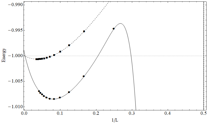
The predicted local minimum of the energy at level 12 is confirmed directly from the data, and the tachyon vev minimum predicted at level 26 is ruled out; the data suggest the minimum is closer to levels 42-46.
The projector-based Newton method is general for linear b-gauges, so high-level numerical solutions can now be searched for in gauges other than Siegel and Schnabl.
The projected-out equations of motion and the symmetry identities of the analytic solution are satisfied asymptotically, which supports calling the numerical solution physical.

Reading between the lines

Editorial extensions of the paper, not claims the author makes directly.

If the instability of the extrapolations is caused by the gauge condition coupling fields at different levels, then other non-diagonal linear b-gauges should show similar or worse convergence as they move away from the Siegel gauge; the same projector method could test this quantitatively.
The two-stage $1/L$-then-$1/N$ extrapolation that works for the tachyon coefficient suggests the finite-level corrections follow a systematic asymptotic expansion; if so, the same procedure could sharpen predictions for all coefficients and for other observables.
The candidate second solution whose energy extrapolates near zero may be a level-truncation artifact or a gauge copy of the vacuum; continuing it to higher levels with the new method would decide which.
The failure of the KBc restricted-space truncation suggests that numerical level truncation cannot be trusted for highly constrained ansatze; a fully analytic treatment is needed there, so any future numerical check of KBc-type solutions would need a different projection.

Share X Bluesky LinkedIn Reddit HN

Signed reviews

No signed human review yet.

Editorial analysis

A structured set of objections, weighed in public.

Desk editor's note, referee report, and a circularity audit.

Desk Editor's Note

read the letter

Short version: this is a genuinely useful numerical methods paper with honest caveats, not a physics breakthrough. The new elements are the canonical-projector Newton method (section 2) that pushes Schnabl-gauge level truncation from L=10 to L=24, and the data that come with it. The infinite-level extrapolations are the weak joint, and the authors mostly know it.

What is actually good. The projector construction is clean and applies to any linear b-gauge; the factorized-vertex handling is the key trick that makes L=24 feasible. They verify the method reproduces the old L≤10 results, so the pipeline is credible. The L=24 energy data in table 4.1 directly show the predicted L=12 local minimum, which settles a specific conjecture from [36]. The finite-level tables look internally consistent, and appendix A's predictive test (fitting lower levels to forecast L=24) is a good check that the data are smooth. The out-of-gauge residual checks are limited to the five dependent variables, but as a spot check they behave sensibly.

Where it gets soft. Everything about L=∞ sits on 1/L polynomial extrapolation, and that load-bearing step is only partially controlled. The energy extrapolants in table 4.2 bounce around in the tail by ~10^-4 to 10^-3; the paper quotes an error of order 10^-4 while the central value sits about 5×10^-4 from -1, so the error estimate is not really earned. The Ellwood invariant is more exposed: the single maximal-order fit of all twelve points gives 3.36, nowhere near zero. The paper recovers a sensible value by splitting into 4k and 4k+2 subsequences and averaging two order-5 fits. That split is not purely invented — the 4-level separation is standard for Ellwood invariants (footnote 5, ref [38]) — but two six-point fits whose limits differ by about a quarter of the answer cannot support the claimed 0.15% precision. Similarly, the N→∞ extrapolations for the tachyon vev use M=5 partly because it lands near the analytic value; the authors admit this is likely coincidental. So the central identification — that the numerical solution converges to Schnabl's analytic vacuum — is supported by converging evidence but not established by controlled error estimates. The paper says as much in section 7, which is to its credit.

Who this is for: anyone doing numerical open string field theory, especially in non-Siegel gauges; the projector method is the reusable takeaway. The physics conclusions are already known analytically, so the value is in the technique and in the L=24 reference data. This deserves a proper referee — the method should be checked and the extrapolation claims tightened. I would also ask the authors to make code and data available, since none are included.

Recommendation: send to peer review with a request to soften the infinite-level precision claims and to justify or remove the post-hoc fit choices.

Referee Report

4 major / 6 minor

Summary. The paper develops a level-truncation-based numerical method for Witten's open bosonic string field theory in the Schnabl gauge, allowing computations up to level L=24, and uses it to study the tachyon vacuum. It reports that the vacuum energy has a local minimum at L=12 (confirming the earlier prediction of [36]) and that extrapolations in 1/L give an infinite-level energy near -0.9995, an Ellwood invariant near -0.0015, and coefficients close to Schnabl's analytic values. The paper also checks K1 matter symmetries and a subset of out-of-gauge equations, and discusses other numerical solutions. The authors conclude that the numerical solution is most likely the infinite-level analytic Schnabl solution, but they explicitly acknowledge partial instability and the possibility that the solution is non-analytic around infinite level.

Significance. If the identification with Schnabl's analytic solution is correct, the paper provides the first high-level numerical confirmation in the Schnabl gauge and a general method for nontrivial linear b-gauges. The finite-level data are valuable and internally consistent: the local minimum at L=12 is visible directly in Table 4.1 without any extrapolation, and the method reproduces the earlier L<=10 results. The paper is also commendably explicit about the limitations of its extrapolations. However, the infinite-level claims are the load-bearing part of the paper and currently rest on extrapolation procedures whose stability is not established, especially for the Ellwood invariant and for the energy.

major comments (4)

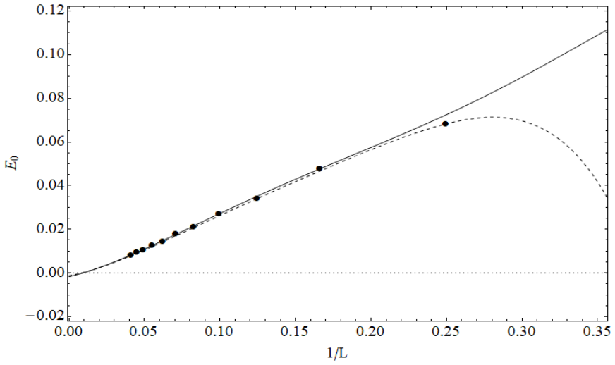
[§4, Eqs. (4.2)–(4.3)] The claimed infinite-level value of the Ellwood invariant E0 is not supported by the data alone. A single maximal-order 1/L fit to all twelve points of Table 4.3 gives 3.3629, which the authors discard; they then split the data into L=4k and L=4k+2 subsequences and fit each with order N=5, obtaining -0.00172 and -0.00129, and average these to -0.0015. This split and fit order are selected after the standard fit fails, and the two subsequence limits differ by about 25% of the final answer. With only six points per subsequence, the statement that E0 is reproduced with 0.15% precision is not established. The authors should present the full set of extrapolants for all choices of Lmin, Lmax, and order M, justify the 4k/4k+2 split independently of the target value, and report a systematic uncertainty that includes the spread of the two subsequence fits.
[§4, Table 4.2 and §7] The energy extrapolation is not stable enough to justify the claimed 10^-4 error. The maximal-order extrapolants E_N(infinity) in Table 4.2 run from -1.0299 (N=1) to -0.999486 (N=11), a spread of about 3×10^-2, and the sequence has not plateaued. Section 7 explicitly concedes that the numerical solution may be a non-analytic function of 1/L, in which case the ansatz (A.1) is not the correct asymptotic expansion. The conclusion that Sen's first conjecture holds at the 0.05% level should be reformulated as a tentative statement, with an uncertainty estimate that includes the spread over extrapolation orders and the possibility of non-polynomial asymptotics.
[§3, Table 3.3] The second, N-to-infinity extrapolation for the string field coefficients is calibrated against the known analytic answer: the degree M=5 is chosen because it best reproduces the analytic tachyon coefficient, and the authors themselves call the resulting 0.01% agreement 'probably coincidental' (Section 3). Since the same M=5 fit yields values for u, v, w, and w1 that are less accurate, the evidence that the numerical coefficients converge to the analytic ones is weaker than the tachyon coefficient alone suggests. Please quantify the dependence on M and report the fit quality for all coefficients without using the known target values as a selection criterion.
[§6, Table 6.1] The out-of-gauge checks cover only fw, fw1, fw2, fw3, and fw4, the five equations associated with the dependent variables at level 4. At higher levels the projector removes many more equations, so these five components do not certify that the full projected-out subspace vanishes asymptotically. The text should state this limitation explicitly, or extend the check to a larger set of out-of-gauge equations.

minor comments (6)

[§2, Eq. (2.17)] The index in the sum should be t(I)_j, not t(I)_i; as written the equation is circular.
[§4, Eq. (4.1)] The notation <V|Psi> and <I|V(i)|Psi> is inconsistent; please define V(i) and the normalization used for the identity string field.
[Table 3.1] The column for w1 is described as 'from level 4', but the first numerical entry appears at L=6; please clarify why the level-2 and level-4 entries are omitted.
[Figure 4.2] Add axis labels and a legend identifying which curve is f5(L) and which is g5(L).
[Appendix A] The use of Mathematica's NonlinearModelFit is implementation-specific; state the least-squares formulation and the handling of numerical precision in a way that makes the procedure reproducible.
[Table 1.1] The tachyon coefficient is listed under the heading c1|0> in Table 1.1 but as t in Section 3; align the notation across the two tables.

Circularity Check

2 steps flagged · score 4.0 of 10

Finite-level data and energy are independent, but the N-to-infinity extrapolation order and the Ellwood-invariant data split are selected after comparing with the known analytic values, so the reported agreement is partially tuned, not fully predicted.

fitted input called prediction [Section 3, paragraph after Table 3.3 (N→∞ extrapolations of tachyon condensate coefficients)]
"By repeating the same analysis for other coeﬃcients, we have reached a conclusion that M = 5 is the best overall choice, so these results are shown in the penultimate row of table 3.1 denoted by N → ∞. For the tachyon coeﬃcient, the result of the M = 5 extrapolation agrees very well with the analytical value."

The order M of the second, N→∞ extrapolation is chosen because it best reproduces the known analytic coefficients, including the tachyon vacuum expectation value t=0.55346558. The same order M=5 is then used to produce the 'N→∞' row of Table 3.1, and the closeness of that row to the analytic row is reported as evidence of convergence. Thus the agreement is partly a consequence of selecting the fit order with the target answer in view, rather than an out-of-sample prediction. The raw level-truncation coefficients are genuine, so this is partial circularity in the extrapolation stage only.
fitted input called prediction [Section 4, paragraph after Table 4.3 (Ellwood invariant E0)]
"However when we compute the asymptotic value L→∞ of this order N = 11 function, we get 3.3629, which is clearly far away from the expected value E0 = 0. ... By taking the average of these two asymptotic values, we get −0.0015, which means that this extrapolation technique gives us the invariant E0 with a relative precision of 0.15%."

The standard maximal-order 1/L fit is abandoned precisely because it does not produce the known analytic value E0=0. The data are then divided into the subsequences L=4k+2 and L=4k, each fitted with order N=5, and the two limits (-0.00172 and -0.00129) are averaged to obtain -0.0015. This data split and fit order are introduced after seeing that the un-split fit fails, with the expected value zero used as the selection criterion. Therefore the reported 0.15% agreement is an artefact of the chosen extrapolation prescription rather than an independent convergence test; the monotone decrease of the raw data is real, but the claimed precision is not forced by the data alone.

full rationale

The central computation is self-contained: the Schnabl-gauge equations are projected with the canonical projector of Section 2 and solved by Newton's method up to level 24, and the raw table entries (energy, coefficients, Ellwood invariant) are not constructed from the analytic solution. The energy data do not have -1 as an input, the local minimum at L=12 is read directly from new data, and the extrapolated energy -0.99949 with its stated uncertainty is an independent numerical result. The symmetry identities of Section 5 and the out-of-gauge equations of Section 6 are also checks against the analytic solution and are not built into the solving procedure. The circularity is confined to the extrapolation stage: the N→∞ fit order M=5 is selected because it best reproduces known analytic values (Section 3), and the Ellwood-invariant extrapolation switches to a split 4k/4k+2 fit only after the standard fit gives 3.3629 instead of 0, so part of the reported agreement is selected rather than predicted. Self-citations to Schnabl [2], Arroyo et al. [36], Kudrna's thesis [38], and Kudrna-Maccaferri [42] provide the formulation and extrapolation techniques, but they are not load-bearing as unverified theorems; the method is partly validated internally by the level-24 predictions in Table A.1. Because the finite-level data and the main energy trend are independent, the paper is not forced by definition, but the tuned extrapolation choices prevent a clean non-circular verdict. Score 4.

Assumptions & free parameters 2 free parameters · 6 assumptions · 0 invented entities

The physical input is the standard SFT framework; no new constants or entities are introduced. The analysis introduces extrapolation fit parameters and relies on untested convergence assumptions; these dominate the uncertainty in the infinite-level claims.

free parameters (2)

Extrapolation polynomial coefficients a0...a_M (1/L fits) = e.g. energy limit -0.99949, tachyon coefficient 0.5457; not physical constants
Least-squares coefficients for the functions (A.1) fitted to level-truncated data; the claimed L to infinity limits are the leading coefficients a0. They are analysis parameters, not theory inputs.
N to infinity fit coefficients r0...r_M and degree M=5 = e.g. tachyon coefficient 0.553396 vs analytic 0.553466
Coefficients of the second extrapolation in 1/N (A.2); degree M=5 is chosen by hand as the best overall choice, partly by agreement with analytic values.

assumptions (6)

domain assumption Witten's cubic open bosonic string field theory action and star product define the dynamics.
The paper solves Q Psi + Psi * Psi = 0 for Witten's OSFT; this framework is taken from the cited literature, not rederived.
domain assumption Level truncation (L,3L) gives a valid finite-dimensional approximation whose solutions converge to the full theory as L goes to infinity.
Assumed throughout; the paper explicitly tests convergence indicators and notes the Schnabl gauge has unusual asymptotic behavior.
domain assumption The canonical projector PC built from the gauge matrix reproduces the equations of the reduced gauge-fixed action at every level.
Shown for a level-4 example and checked against [36] up to level 10; used for all levels up to 24.
ad hoc to paper The numerical solution on the projected equations lies on the branch that connects to Schnabl's analytic solution.
This is the conjecture the paper tests; consistency checks support it but do not prove branch selection.
ad hoc to paper Extrapolations of the form (A.1) and (A.2) capture the asymptotic behavior of level-truncated quantities.
Not established; the authors caution the solution could be non-analytic around level infinity, which would invalidate polynomial extrapolation.
domain assumption Equations projected out by the gauge choice vanish asymptotically.
The paper checks several out-of-gauge equations and finds approximate decay, but assumes exact asymptotic vanishing for the consistency of the approach.

how reviews work

0 comments

Cite this review

Pith. "Pith review of Numerical solution for tachyon vacuum in the Schnabl gauge." pith.science (2026). https://pith.science/paper/WCYJ3UUF

@misc{pith2026190805330,
  author       = {Pith},
  title        = {Pith review of: Numerical solution for tachyon vacuum in the Schnabl gauge},
  year         = {2026},
  howpublished = {\url{https://pith.science/paper/WCYJ3UUF}},
  note         = {Machine review of arXiv:1908.05330}
}

abstract

Based on the level truncation scheme, we develop a new numerical method to evaluate the tachyon vacuum solution in the Schnabl gauge up to level $L=24$. We confirm the prediction that the energy associated to this numerical solution has a local minimum at level $L=12$. Extrapolating the energy data of $L \leq 24$ to infinite level, we observe that the energy goes towards the analytical value $-1$, nevertheless the precision of the extrapolation is lower than in the Siegel gauge. Furthermore, we analyze the Ellwood invariant and show that its value converges monotonically towards the expected analytical result. We also study the tachyon vacuum expectation value (vev) and some other coefficients of the solution. Finally, some consistency checks of the solution are performed, and we briefly discuss the search for other Schnabl gauge numerical solutions.

Figures

Figures reproduced from arXiv: 1908.05330 by the authors.

**Figure 3.1.** The tachyon coefficient data up to level [PITH_FULL_IMAGE:figures/full_fig_p014_3_1.png] view at source ↗

**Figure 4.1.** Data for the energy in the Schnabl gauge as well as in the Siegel gauge as a [PITH_FULL_IMAGE:figures/full_fig_p016_4_1.png] view at source ↗

**Figure 4.2.** Data for the gauge invariant quantity E0 up to level L = 24 in the Schnabl gauge as a function of 1/L. The solid curve represents the function f5(L), while the dashed curve represents the function g5(L). The dotted line represents the expected analytical value E0 = 0. extrapolate levels 4k + 2 and 4k separately5 . Namely, we divide the twelve data points of table 4.3 into two sets of six data points, the ones at lev… view at source ↗

Discussion (0). Continue with ORCID to comment.

Reference graph

Works this paper leans on

45 extracted references · 22 canonical work pages

[36]

Numerical solution of open string field theory in Schnabl gauge

E. A. Arroyo, A. Fernandes-Silva and R. Szitas, “Numerical solution of open string ﬁeld theory in Schnabl gauge,” JHEP1801, 007 (2018) doi:10.1007/JHEP01(2018)007 [arXiv:1707.09452 [hep-th]]

work page Pith review arXiv 2018
[38]

Level Truncation Approach to Open String Field Theory,

M. Kudrna, “Level Truncation Approach to Open String Field Theory,” Ph.D. the- sis, https://dspace.cuni.cz/bitstream/handle/20.500.11956/110558/140080054. pdf

work page
[1]

Noncommutative Geometry and String Field Theory,

E. Witten, “Noncommutative Geometry and String Field Theory,” Nucl. Phys. B 268, 253 (1986). doi:10.1016/0550-3213(86)90155-0

doi:10.1016/0550-3213(86)90155-0 1986
[2]

Analytic solution for tachyon condensation in open string ﬁeld theory,

M. Schnabl, “Analytic solution for tachyon condensation in open string ﬁeld theory,” Adv. Theor. Math. Phys. 10, no. 4, 433 (2006) doi:10.4310/ATMP.2006.v10.n4.a1 [hep-th/0511286]

arXiv 2006
[3]

Descent relations among bosonic D-branes,

A. Sen, “Descent relations among bosonic D-branes,” Int. J. Mod. Phys. A 14, 4061 (1999) doi:10.1142/S0217751X99001901 [hep-th/9902105]

arXiv 1999
[4]

Universality of the tachyon potential,

A. Sen, “Universality of the tachyon potential,” JHEP9912, 027 (1999) doi:10.1088/1126- 6708/1999/12/027 [hep-th/9911116]

arXiv 1999
[5]

Comments on Schnabl’s analytic solution for tachyon condensation in Witten’s open string ﬁeld theory,

Y. Okawa, “Comments on Schnabl’s analytic solution for tachyon condensation in Witten’s open string ﬁeld theory,” JHEP 0604, 055 (2006) doi:10.1088/1126- 6708/2006/04/055 [hep-th/0603159]

arXiv 2006
[6]

Analytic methods in open string ﬁeld theory,

Y. Okawa, “Analytic methods in open string ﬁeld theory,” Prog. Theor. Phys. 128, 1001 (2012). doi:10.1143/PTP.128.1001

work page doi:10.1143/ptp.128.1001 2012

Show all 45 references

[7]

Schnabl’s L(0) operator in the continuous basis,

E. Fuchs and M. Kroyter, “Schnabl’s L(0) operator in the continuous basis,” JHEP 0610, 067 (2006) doi:10.1088/1126-6708/2006/10/067 [hep-th/0605254]

2006 arXiv
[8]

Conservation laws and tachyon potentials in the sliver frame,

E. A. Arroyo, “Conservation laws and tachyon potentials in the sliver frame,” JHEP 1106, 033 (2011) doi:10.1007/JHEP06(2011)033 [arXiv:1103.4830 [hep-th]]

2011 arXiv
[9]

Solving Open String Field Theory with Special Projec- tors,

L. Rastelli and B. Zwiebach, “Solving Open String Field Theory with Special Projec- tors,” JHEP 0801, 020 (2008) doi:10.1088/1126-6708/2008/01/020 [hep-th/0606131]

2008 arXiv
[10]

Proof of vanishing cohomology at the tachyon vacuum,

I. Ellwood and M. Schnabl, “Proof of vanishing cohomology at the tachyon vacuum,” JHEP 0702, 096 (2007) doi:10.1088/1126-6708/2007/02/096 [hep-th/0606142]

2007 arXiv
[11]

Analytic Solutions for Tachyon Conden- sation with General Projectors,

Y. Okawa, L. Rastelli and B. Zwiebach, “Analytic Solutions for Tachyon Conden- sation with General Projectors,” hep-th/0611110

arXiv
[12]

Split String Formalism and the Closed String Vacuum,

T. Erler, “Split String Formalism and the Closed String Vacuum,” JHEP 0705, 083 (2007) doi:10.1088/1126-6708/2007/05/083 [hep-th/0611200]

2007 arXiv
[13]

Split String Formalism and the Closed String Vacuum, II,

T. Erler, “Split String Formalism and the Closed String Vacuum, II,” JHEP 0705, 084 (2007) doi:10.1088/1126-6708/2007/05/084 [hep-th/0612050]

2007 arXiv
[14]

Algebraic solutions in Open String Field Theory - A Lightning Re- view,

M. Schnabl, “Algebraic solutions in Open String Field Theory - A Lightning Re- view,” Acta Polytechnica 50, no. 3 (2010) 102 [arXiv:1004.4858 [hep-th]]

2010 arXiv
[15]

Analytical Solutions of Open String Field Theory,

E. Fuchs and M. Kroyter, “Analytical Solutions of Open String Field Theory,” Phys. Rept. 502, 89 (2011) doi:10.1016/j.physrep.2011.01.003 [arXiv:0807.4722 [hep-th]]

2011 arXiv
[16]

Linear b-Gauges for Open String Fields,

M. Kiermaier, A. Sen and B. Zwiebach, “Linear b-Gauges for Open String Fields,” JHEP 0803, 050 (2008) doi:10.1088/1126-6708/2008/03/050 [arXiv:0712.0627 [hep- th]]. 29

2008 arXiv
[17]

Level truncation analysis of exact solutions in open string ﬁeld the- ory,

T. Takahashi, “Level truncation analysis of exact solutions in open string ﬁeld the- ory,” JHEP 0801, 001 (2008) doi:10.1088/1126-6708/2008/01/001 [arXiv:0710.5358 [hep-th]]

2008 arXiv
[18]

On numerical solutions in open string ﬁeld theory,

I. Kishimoto, “On numerical solutions in open string ﬁeld theory,” Prog. Theor. Phys. Suppl. 188, 155 (2011). doi:10.1143/PTPS.188.155

2011 doi
[19]

Cubic interaction term for Schnabl’s solution using Pade approxi- mants,

E. A. Arroyo, “Cubic interaction term for Schnabl’s solution using Pade approxi- mants,” J. Phys. A42, 375402 (2009) doi:10.1088/1751-8113/42/37/375402 [arXiv:0905.2014 [hep-th]]

2009 arXiv
[20]

Level truncation analysis of regularized identity based solutions,

E. Aldo Arroyo, “Level truncation analysis of regularized identity based solutions,” JHEP 1111, 079 (2011) doi:10.1007/JHEP11(2011)079 [arXiv:1109.5354 [hep-th]]

2011 arXiv
[21]

Comments on regularization of identity based solutions in string ﬁeld theory,

E. A. Arroyo, “Comments on regularization of identity based solutions in string ﬁeld theory,” JHEP 1011, 135 (2010) doi:10.1007/JHEP11(2010)135 [arXiv:1009.0198 [hep-th]]

2010 arXiv
[22]

Marginal and scalar solutions in cubic open string ﬁeld theory,

T. Takahashi and S. Tanimoto, “Marginal and scalar solutions in cubic open string ﬁeld theory,” JHEP 0203, 033 (2002) doi:10.1088/1126-6708/2002/03/033 [hep- th/0202133]

2002
[23]

A Simple Analytic Solution for Tachyon Condensation,

T. Erler and M. Schnabl, “A Simple Analytic Solution for Tachyon Condensation,” JHEP 0910, 066 (2009) doi:10.1088/1126-6708/2009/10/066 [arXiv:0906.0979 [hep- th]]

2009 arXiv
[24]

Multibrane Solutions in Open String Field Theory,

M. Murata and M. Schnabl, “Multibrane Solutions in Open String Field Theory,” JHEP 1207, 063 (2012) doi:10.1007/JHEP07(2012)063 [arXiv:1112.0591 [hep-th]]

2012 arXiv
[25]

Comments on new multiple-brane solutions based on Hata-Kojita dual- ity in open string ﬁeld theory,

T. Masuda, “Comments on new multiple-brane solutions based on Hata-Kojita dual- ity in open string ﬁeld theory,” JHEP1405, 021 (2014) doi:10.1007/JHEP05(2014)021 [arXiv:1211.2649 [hep-th], arXiv:1211.2649]

2014 arXiv
[26]

Singularities in K-space and Multi-brane Solutions in Cu- bic String Field Theory,

H. Hata and T. Kojita, “Singularities in K-space and Multi-brane Solutions in Cu- bic String Field Theory,” JHEP 1302, 065 (2013) doi:10.1007/JHEP02(2013)065 [arXiv:1209.4406 [hep-th]]

2013 arXiv
[27]

Constraints on a class of classical solutions in open string ﬁeld theory,

T. Masuda, T. Noumi and D. Takahashi, “Constraints on a class of classical solutions in open string ﬁeld theory,” JHEP 1210, 113 (2012) doi:10.1007/JHEP10(2012)113 [arXiv:1207.6220 [hep-th]]

2012 arXiv
[28]

Analytic solutions for Dp branes in SFT,

L. Bonora, S. Giaccari and D. D. Tolla, “Analytic solutions for Dp branes in SFT,” JHEP 1112, 033 (2011) doi:10.1007/JHEP12(2011)033 [arXiv:1106.3914 [hep-th]]

2011 arXiv
[29]

The energy of the analytic lump solution in SFT,

L. Bonora, S. Giaccari and D. D. Tolla, “The energy of the analytic lump solution in SFT,” JHEP 1108, 158 (2011) Erratum: [JHEP 1204, 001 (2012)] doi:10.1007/JHEP08(2011)158, 10.1007/JHEP04(2012)001 [arXiv:1105.5926 [hep-th]]

2011 arXiv
[30]

Analytic solutions for marginal deformations in open string ﬁeld theory,

M. Kiermaier, Y. Okawa, L. Rastelli and B. Zwiebach, “Analytic solutions for marginal deformations in open string ﬁeld theory,” JHEP0801, 028 (2008) doi:10.1088/1126- 6708/2008/01/028 [hep-th/0701249 [HEP-TH]]. 30

2008 arXiv
[31]

String ﬁeld representation of the Virasoro algebra,

N. Mertes and M. Schnabl, “String ﬁeld representation of the Virasoro algebra,” JHEP 1612, 151 (2016) doi:10.1007/JHEP12(2016)151 [arXiv:1610.00968 [hep-th]]

2016 arXiv
[32]

Real Tachyon Vacuum Solution without Square Roots,

M. Jokel, “Real Tachyon Vacuum Solution without Square Roots,” arXiv:1704.02391 [hep-th]

arXiv
[33]

Comments on real tachyon vacuum solution without square roots,

E. A. Arroyo, “Comments on real tachyon vacuum solution without square roots,” JHEP 1801, 006 (2018) doi:10.1007/JHEP01(2018)006 [arXiv:1706.00336 [hep-th]]

2018 arXiv
[34]

Level truncation and the tachyon in open bosonic string ﬁeld theory,

N. Moeller and W. Taylor, “Level truncation and the tachyon in open bosonic string ﬁeld theory,” Nucl. Phys. B 583, 105 (2000) doi:10.1016/S0550-3213(00)00293-5 [hep-th/0002237]

2000 arXiv
[35]

Experimental string ﬁeld theory,

D. Gaiotto and L. Rastelli, “Experimental string ﬁeld theory,” JHEP 0308, 048 (2003) doi:10.1088/1126-6708/2003/08/048 [hep-th/0211012]

2003 arXiv
[37]

Universal Solutions in Open String Field Theory,

M. Kudrna and M. Schnabl, “Universal Solutions in Open String Field Theory,” arXiv:1812.03221 [hep-th]

arXiv
[39]

Numerical Evaluation of Gauge Invariants for a- gauge Solutions in Open String Field Theory,

I. Kishimoto and T. Takahashi, “Numerical Evaluation of Gauge Invariants for a- gauge Solutions in Open String Field Theory,” Prog. Theor. Phys. 121 (2009) 695 doi:10.1143/PTP.121.695 [arXiv:0902.0445 [hep-th]]

2009 arXiv
[40]

Numerical Evaluation of Gauge Invariants for a- gauge Solutions in Open String Field Theory,

I. Kishimoto and T. Takahashi, “Numerical Evaluation of Gauge Invariants for a- gauge Solutions in Open String Field Theory,” Theor. Math. Phys. 163 (2010) 710 doi:10.1007/s11232-010-0054-y [arXiv:0910.3025 [hep-th]]

2010 arXiv
[41]

Tachyon condensation in string ﬁeld theory,

A. Sen and B. Zwiebach, “Tachyon condensation in string ﬁeld theory,” JHEP0003 (2000) 002 doi:10.1088/1126-6708/2000/03/002 [hep-th/9912249]

2000 arXiv
[42]

BCFT moduli space in level truncation,

M. Kudrna and C. Maccaferri, “BCFT moduli space in level truncation,” JHEP 1604, 057 (2016) doi:10.1007/JHEP04(2016)057 [arXiv:1601.04046 [hep-th]]

2016 arXiv
[43]

Observables of string ﬁeld theory,

A. Hashimoto and N. Itzhaki, “Observables of string ﬁeld theory,” JHEP 0201, 028 (2002) doi:10.1088/1126-6708/2002/01/028 [hep-th/0111092]

2002 arXiv
[44]

The Closed string tadpole in open string ﬁeld theory,

I. Ellwood, “The Closed string tadpole in open string ﬁeld theory,” JHEP 0808, 063 (2008) doi:10.1088/1126-6708/2008/08/063 [arXiv:0804.1131 [hep-th]]

2008 arXiv
[45]

Boundary State from Ellwood In- variants,

M. Kudrna, C. Maccaferri and M. Schnabl, “Boundary State from Ellwood In- variants,” JHEP 1307 (2013) 033 doi:10.1007/JHEP07(2013)033 [arXiv:1207.4785 [hep-th]]. 31

2013 arXiv

Pith tools

Reviewed August 14, 2026 · model on record in the stance chip above.

[1] [36]

Numerical solution of open string field theory in Schnabl gauge

E. A. Arroyo, A. Fernandes-Silva and R. Szitas, “Numerical solution of open string ﬁeld theory in Schnabl gauge,” JHEP1801, 007 (2018) doi:10.1007/JHEP01(2018)007 [arXiv:1707.09452 [hep-th]]

work page Pith review arXiv 2018

[2] [38]

Level Truncation Approach to Open String Field Theory,

M. Kudrna, “Level Truncation Approach to Open String Field Theory,” Ph.D. the- sis, https://dspace.cuni.cz/bitstream/handle/20.500.11956/110558/140080054. pdf

work page

[3] [1]

Noncommutative Geometry and String Field Theory,

E. Witten, “Noncommutative Geometry and String Field Theory,” Nucl. Phys. B 268, 253 (1986). doi:10.1016/0550-3213(86)90155-0

doi:10.1016/0550-3213(86)90155-0 1986

[4] [2]

Analytic solution for tachyon condensation in open string ﬁeld theory,

M. Schnabl, “Analytic solution for tachyon condensation in open string ﬁeld theory,” Adv. Theor. Math. Phys. 10, no. 4, 433 (2006) doi:10.4310/ATMP.2006.v10.n4.a1 [hep-th/0511286]

arXiv 2006

[5] [3]

Descent relations among bosonic D-branes,

A. Sen, “Descent relations among bosonic D-branes,” Int. J. Mod. Phys. A 14, 4061 (1999) doi:10.1142/S0217751X99001901 [hep-th/9902105]

arXiv 1999

[6] [4]

Universality of the tachyon potential,

A. Sen, “Universality of the tachyon potential,” JHEP9912, 027 (1999) doi:10.1088/1126- 6708/1999/12/027 [hep-th/9911116]

arXiv 1999

[7] [5]

Comments on Schnabl’s analytic solution for tachyon condensation in Witten’s open string ﬁeld theory,

Y. Okawa, “Comments on Schnabl’s analytic solution for tachyon condensation in Witten’s open string ﬁeld theory,” JHEP 0604, 055 (2006) doi:10.1088/1126- 6708/2006/04/055 [hep-th/0603159]

arXiv 2006

[8] [6]

Analytic methods in open string ﬁeld theory,

Y. Okawa, “Analytic methods in open string ﬁeld theory,” Prog. Theor. Phys. 128, 1001 (2012). doi:10.1143/PTP.128.1001

work page doi:10.1143/ptp.128.1001 2012