REVIEW 3 major objections 6 minor 35 references
Quantum Cosmology with many fluids and the choice of cosmological time
T0 review · 3 major / 6 minor · reviewed 2026-08-14 · deepseek-v4-flash
Pith's one-line read This paper claims that in a quantized closed universe filled with five barotropic fluids, the vacuum fluid is the only viable choice of physical time because it alone produces a tunneling transition from the Planck era to classical…
desk verdict A competent five-fluid minisuperspace construction whose vacuum-time conclusion rests on a tunneling probability that is not actually a tunneling probability. read the letter →
The pith
A machine-rendered reading of the paper's core claim, the machinery that carries it, and where it could break.
The reading
What carries the argument
The key machinery is the Schutz velocity-potential formalism for perfect fluids, which makes the conjugate momentum of a fluid potential appear linearly in the super-Hamiltonian, so that after canonical quantization one obtains a time-dependent Schrödinger equation with the fluid variable as time. For the vacuum ($\omega = -1$) case, the equation initially has a time-derivative term multiplied by $a^4$, but a canonical change of variable to $x$ recasts it as a standard Schrödinger equation with an effective potential $V_{\rm ef}(x)$ that has a small barrier. The numerical workhorse is the Crank–Nicolson finite-difference method, used to evolve the initial packet and to compute the tunneling probability $TP = \int_{x_2}^{x_f} |\Psi(x,t_f)|^2 dx \,/\, \int_0^{x_f} |\Psi(x,t_f)|^2 dx$, where $x_2$ is the right turning point of the barrier.
What would settle it
Evolve the same initial packet with its center shifted from $x \approx 0.189$ to a position clearly to the left of the barrier turning point $x_1 \approx 0.095$, and compute the transmitted fraction $\int_{x_2}^{65} |\Psi|^2 dx$ at $t_f = 10$; if this fraction falls to the order of the WKB values in Table 2, the near-unity tunneling probability is an artifact of launching the packet inside the forbidden region.
Extended reading notes
Core claim
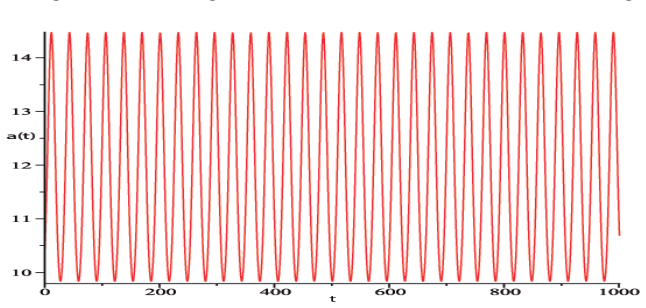
Within the Schutz formalism, each fluid choice turns the Wheeler–DeWitt equation into a Schrödinger equation with that fluid's canonical momentum as time. The paper finds that radiation, dust, cosmic strings, and domain walls all yield bound-state spectra; their wave packets are normalizable, remain well-defined at $a \to 0$, and give expectation values of the scale factor that oscillate inside the classical oscillation region. The vacuum case is qualitatively different: after a canonical transformation to a new variable $x$, the effective potential becomes a small potential barrier rather than a well. Evolving a wave packet with energy $E_m = 3.5$ just below the barrier top through the Crank–Nicolson method gives a tunneling probability $TP \approx 1$ (and $TP \geq 0.98$ for $E_m \geq 0.5$), compared with WKB estimates below 0.6. The expected scale factor contracts slightly, never vanishes, and then expands, matching the classical trajectory after tunneling. The paper's central conclusion is that vacuum is the only one of the five fluids that provides a quantum-to-classical transition, and therefore the best choice for the role of time.
Load-bearing premise
The near-unity tunneling probability rests on the assumption that the initial wave packet (43), with $E_m = 3.5$, is the correct pre-tunneling state, even though its maximum lies inside the potential barrier rather than in the classically allowed region to the left.
Editorial extensions
If this is right
- If the vacuum-fluid time choice is correct, the universe emerges from the Planck era by tunneling through a small potential barrier into a classically expanding state, with no singularity at $a = 0$.
- The near-unity tunneling probability ($TP \geq 0.998$ for $E_m \geq 0.6$) means the quantum-to-classical transition is essentially certain for a wide range of initial energies below the barrier top.
- For radiation, dust, cosmic strings, and domain walls, the quantized universe would oscillate forever within a bounded range of scale factors, with no transition to a classical expanding phase, so those fluids are poor time variables.
- The expected value of the scale factor in the vacuum case is always nonzero, providing a singularity-free description of the primordial universe.
- The vacuum case yields a continuous energy spectrum, in contrast to the discrete bound states of the other fluids, which is why a different numerical method (Crank–Nicolson) is required.
Reading between the lines
- If the vacuum-time result is taken at face value, the model predicts that the universe's classical expansion begins only after a tunneling event, so the Planck era is connected to the classical phase by a continuous quantum process with no singularity; this is a concrete realization of the tunneling proposal in a multi-fluid setting.
- The four non-vacuum fluid-time choices produce bouncing, oscillating universes; a natural next test is whether any of those oscillations could be observationally distinguished from the standard expanding history, which would strengthen or weaken the case for vacuum time.
- The computation's sensitivity to the initial packet placement suggests a direct extension: repeat the evolution with packets of different widths and centers, and compare the transmitted fraction with the WKB formula, to map the conditions under which $TP \approx 1$ actually holds.
Signed reviews
Editorial analysis
A structured set of objections, weighed in public.
Referee Report
Summary. The paper quantizes a closed FLRW minisuperspace model with five non-interacting barotropic fluids (radiation, dust, cosmic strings, domain walls, vacuum) in Schutz's formalism. For each fluid chosen as the time variable it obtains a reduced dynamics, solves the bound-state problems for four fluids with the Galerkin spectral method and the vacuum case with a Crank-Nicolson finite-difference scheme, and compares quantum expectation values with classical trajectories. Its central claim is that the vacuum fluid is the best time variable because it is the only one that gives a quantum-to-classical transition via tunneling, with probability near unity.
Significance. The extension from one- or two-fluid models to five fluids is a useful exercise, and the spectral data in Table 1 plus the numerical details (N, dt, xf) make the calculations reproducible. If the tunneling claim were correct, the paper would offer a concrete phenomenological criterion for choosing a fluid time variable in quantum cosmology. As it stands, however, the main conclusion depends on a misidentification of the quantity in Eq. (44) as a tunneling probability and on hand-picked energies; those issues are load-bearing rather than cosmetic.
major comments (3)
- [Sec. 3.1, Eqs. (43)-(44)] The quantity TP defined in Eq. (44) is not a tunneling probability. The initial packet (43) is real, so it has zero mean momentum and is not an incoming wave from the left; for the value Em=3.5 used in the main calculation its maximum lies at x about 0.189, inside the forbidden interval x1=0.0953, x2=0.2223 given in Table 2, with a substantial part of the initial normalization already to the right of x2. Equation (44) then measures the fraction of probability in the classically allowed region at the fixed time tf=10, which combines initially transmitted probability, spreading from inside the barrier, and possible boundary effects at xf=65, rather than a transmitted flux. Because the conclusion in Sec. 4 that the vacuum is the unique time variable with a tunneling transition rests entirely on TP, the central claim is unsupported.
- [Table 2 and Sec. 3.1, parameter values] The near-unity result is selected by the parameter choices rather than derived. The barrier in Eq. (42) is built from hand-assigned fluid energies Ev=-0.0017, Ed=1/24, Edw=1/24, Er=1/24 and Ecs=5.75, and the initial packet energy is chosen as Em=3.5, just below Vef(xmax)=3.803. The same Table 2 shows that TP drops to 0.181 at Em=0.3 and to 4.33e-12 at Em=0.1, while the WKB column changes by eight orders of magnitude over the same range. The agreement of TP with the WKB transmission coefficient is also poor (TP=1.000 versus 0.599 at Em=3.5), reflecting that the two quantities measure different processes. A robust claim about 'tunneling probability near one' needs a physical justification for Em and for the fluid energies, not a regime chosen after the fact.
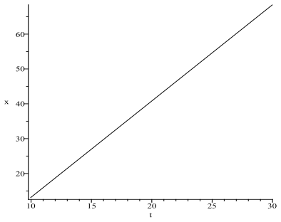
- [Sec. 3.3, Eq. (50) and Fig. 13] The matching of the quantum expectation value to the classical trajectory is not established. Eq. (50) gives x(9.95)=13.03390565 and x'(9.95)=2.763117600, while the caption of Fig. 13 states x(10)=65 and x'(10)=2.763117600; these initial data are mutually inconsistent and the value 65 coincides with the numerical boundary xf. The paper does not explain how the classical initial data are obtained from the wave packet or why a matching at a single time at the boundary is sufficient to demonstrate that the universe 'emerges classically' after tunneling. This weakens the comparison with classical dynamics that supports the final conclusion.
minor comments (6)
- [Sec. 3.1] The sentence 'According to the effective potential described by Eq. (24)' should refer to Eq. (42), since Eq. (24) is the cosmic-strings potential in a, not the vacuum potential in x.
- [Eq. (22)] The right-hand side of Eq. (22) contains partial derivatives with respect to t_j, but the left-hand side is written with t_m; the notation should be made consistent by using t_m on both sides.
- [Abstract and Sec. 1] The formalism name appears as 'Schultz' in the Abstract and Sec. 1; it should be 'Schutz', as used in the references and the rest of the text.
- [Sec. 2, Galerkin calculations] The choice of L=15 or L=5 in the Galerkin calculations is not justified, and the dependence of the eigenvalues in Table 1 on L is not discussed; this matters because the energy eigenvalues enter the classical momentum assignments.
- [Sec. 3.2] The statement that <x>(t) is nonzero 'for all t' is inferred from a numerical evolution to tf=10 in a finite box; the paper should state that this is a numerical result and not an analytic proof of singularity avoidance.
- [Sec. 3.1, Eq. (46)] The energy E appearing in Eq. (46) is never defined explicitly; the authors should state whether it is the initial packet energy Em and explain how the WKB values in Table 2 are obtained from the expression.
Circularity Check
No circularity found: the tunneling-probability result is parameter-sensitive and the TP measure is contestable, but no prediction reduces to its inputs by construction or via a self-citation chain.
full rationale
The derivation chain is self-contained in the sense required: the Hamiltonian (15)-(17), the Wheeler-DeWitt equation (20), and the five time-dependent Schrödinger equations (22)-(42) are obtained from the Schutz action by stated substitutions and canonical transformations, not by importing the conclusion. The canonical transformation (39) and the Crank-Nicolson implementation are taken from earlier works that include the present authors, but the transformation is stated explicitly and is algebraically checkable, so the self-citation is not load-bearing in a circular way. The tunneling probability formula (44) is also quoted from [32], yet it is written out in full; the numerical values in Table 2 follow from that formula, the potential (42), and the initial packet (43), rather than from an unexamined self-cited theorem. The main scientific weakness is that Eq. (44) is a right-of-barrier fraction at a single final time, and for Em=3.5 the packet (43) is centered inside the forbidden region, so the reported TP≈1 is not a standard barrier-transmission probability and is sensitive to the chosen Em and box size. That is a correctness and interpretation concern about what is being computed, not a circular reduction of the prediction to the input; the paper's conclusion is not forced by a definition, by fitting to data, or by a self-citation chain. Accordingly, the circularity score is 0.
Assumptions & free parameters
free parameters (5)
- Ev (vacuum momentum p_Tv) =
-0.0017
- Ed, Ecs, Edw, Er (other fluid energies) =
1/24 each
- Ecs = pTcs for the vacuum potential =
5.75
- Em (initial wave-packet energy) =
3.5
- Numerical box and truncation =
L=15 (or 5), xf=65, N=4500, dt=0.05, tf=10, 10 lowest states
assumptions (5)
- domain assumption Schutz's velocity-potential formalism correctly describes a barotropic perfect fluid and provides a canonical time variable.
- domain assumption All five fluids are non-interacting and each obeys p = omega*rho with constant omega.
- ad hoc to paper For the fluid not chosen as time, its momentum is an unquantized constant with a continuum spectrum whose value can be assigned by hand.
- domain assumption The Wheeler-DeWitt equation with weight a^(1-3*omega) can be solved by the Galerkin method on a finite interval with boundary conditions Psi(0)=Psi(L)=0, and ten states suffice.
- ad hoc to paper The initial packet (43), placed inside or at the barrier with energy Em below Vmax, represents quantum-to-classical tunneling, and TP as defined by Eq. (44) measures tunneling probability.
Cite this review
Pith. "Pith review of Quantum Cosmology with many fluids and the choice of cosmological time." pith.science (2026). https://pith.science/paper/I6S5WTPC
@misc{pith2026190805337,
  author       = {Pith},
  title        = {Pith review of: Quantum Cosmology with many fluids and the choice of cosmological time},
  year         = {2026},
  howpublished = {\url{https://pith.science/paper/I6S5WTPC}},
  note         = {Machine review of arXiv:1908.05337}
}
read the original abstract
In this work we propose the quantization of a cosmological model describing the primordial universe filled with five barotropic fluids, namely: radiation, dust, vacuum, cosmic strings and domain walls. We intend to identify which fluid is best suited to provide phenomenologically the temporal variable in accordance with the observable universe. Through the Galerkin spectral method and the finite difference method in the Crank-Nicolson scheme (vacuum case), the quantum cosmological solutions are obtained and compared. We, also, compare the quantum cosmological solutions with the corresponding classical ones. The vacuum case is especially interesting because it provides a tunneling transition mechanism from the quantum to the classical phase and the possibility of calculating quantum tunneling probabilities.
Figures


Figures from the paper (10 more)




Reference graph
Works this paper leans on
-
[1]
J.J. Halliwell, Introductory Lectures on Quantum Cosmology , in Pro- ceedings of the 7th Jerusalem Winter School for Theoretical Physics, Jerusalem, Israel, edited by S. Coleman, J. Hartle, T. Piran, S. Wein- berg (World Scientific, Singapore, 1991)
work page 1991
-
[2]
R. Arnowitt, S. Deser and C.W. Misner, The Dynamics of General Relativity, in Gravitation: An Introduction to Current Research, edited by L. Witten (Wiley, New York, 1962)
work page 1962
-
[3]
E. Anderson, The Problem of Time in Quantum Gravity , in Classical and Quantum Gravity: Theory, Analysis and Applications, edited by V.R. Frignanni (Nova Science Pub Inc, UK, 2012)
work page 2012
- [4]
-
[5]
F.G. Alvarenga, R.G. Furtado, R. Fracalossi and S.V.B. Gonçalves, Braz. J. Phys.47, 96 (2016)
work page 2016
-
[6]
F.G. Alvarenga, J.C. Fabris, N.A. Lemos and G.A. Monerat , Gen. Relativ. Gravit. 34, 651 (2002)
work page 2002
-
[7]
G.A. Monerat, G. Oliveira-Neto, E.V. Corrêa Silva, L.G. Ferreira Filho, P. Romildo Jr., J.C. Fabris, R. Fracalossi, S.V.B. Gonçalves and F.G. Alvarenga. Phys. Rev. D76, 024017 (2007)
work page 2007
-
[8]
R.C. Freitas, G.A. Monerat, G. Oliveira-Neto, F.G. Alvarenga, S.V.B. Gonçalves, R. Fracalossi, E.V. Corrêa Silva and L.G. Ferreira Filho, Physics of the Dark Universe25, 100325 (2019)
work page 2019
Show all 35 references
-
[9]
Alvarenga, R.C
F.G. Alvarenga, R.C. Freitas, R. Fracalossi and S.V.B. Gonçalves, Gen. Relativ. Gravit. 49, p. 136 (2017)
2017
-
[10]
Pinto-Neto, E
N. Pinto-Neto, E. Sergio Santini and F.T. Falciano, Phys Lett.A, 344 (2005)
2005
-
[11]
Hindmarsh and T.W.B
M.B. Hindmarsh and T.W.B. Kibble, Rep. Prog. Phys.58, 477 (1995)
1995
-
[12]
Copeland and T.W.B
E.J. Copeland and T.W.B. Kibble, Proc. R. Soc.A, 466 (2010)
2010
-
[13]
Vachaspati and A
T. Vachaspati and A. Vilekin, Phys. Rev. Lett.67, 1057 (1991)
1991
-
[14]
Jeong and G.F
E. Jeong and G.F. Smoot, APJ624, 21 (2005). 25
2005
-
[15]
Sarangi and S
S. Sarangi and S. Tye, Phys. Lett. B536, 185 (2002)
2002
-
[16]
Copeland, R.C
E. Copeland, R.C. Myers and J. Polchinski, J. High Energy Phys. JHEP06 013 (2004)
2004
-
[17]
Sakellariadou, J
M. Sakellariadou, J. Cosmol. Astropart. Phys. JCAP04 003 (2005)
2005
-
[18]
Blanco-Pillado, K.D
J.J. Blanco-Pillado, K.D. Olum and X. Siemens, Phys. Lett. B778, 392 (2018)
2018
-
[19]
Battye and A
R. Battye and A. Moss, Phys. Rev. D82, 023521 (2010)
2010
-
[20]
Silva, G.A
E.V.C. Silva, G.A. Monerat, G. de Oliveira Neto and L.G. Ferreira Filho, Comput. Phy. Commun.185, 380 (2014)
2014
-
[21]
Boyd, Chebyshev and Fourier Spectral Methods, second ed., Dover, New York, 2001
J.P. Boyd, Chebyshev and Fourier Spectral Methods, second ed., Dover, New York, 2001
2001
-
[22]
Rubakov and M
V.A. Rubakov and M. E. Shaposhnikov, Phys. Lett. B125, 139 (1983)
1983
-
[23]
Dorigoni and D
D. Dorigoni and D. Tong, J. High Energ. Phys. JHEP08 119 (2014)
2014
-
[24]
Fabris and S.V.B
J.C. Fabris and S.V.B. Gonçalves, Braz. J. Phys.33, 834 (2003)
2003
-
[25]
Coles and F
P. Coles and F. Lucchin, Cosmology: The Origin and Evolution of Cosmic Structure (John Wiley & Sons, New York 2002)
2002
-
[26]
Bertone, D
G. Bertone, D. Hooper and J. Silk, Phys. Rep.405, 279 (2005)
2005
-
[27]
G. A. Monerat, E.V.C. Silva, G. Oliveira-Neto, L.G.F. Filho, N.A. Lemos, Braz. J. Phys.35, 1106 (2005)
2005
-
[28]
Atkatz, American Journal Physics62, 619 (1994)
D. Atkatz, American Journal Physics62, 619 (1994)
1994
-
[29]
Peebles and Bharat Ratra, Rev
P.J.E. Peebles and Bharat Ratra, Rev. Mod. Phys.75, 559 (2003)
2003
-
[30]
Crank and P.A
J. Crank and P.A. Nicolson, Advances in Computational Mathematics 6, 207 (I996)
-
[31]
Corrêa Silva, G.A
E.V. Corrêa Silva, G.A. Monerat, G. Oliveira-Neto, C. Neves and L.G. Ferreira Filho, Phys. Rev. D80, 047302 (2009)
2009
-
[32]
Acacio de Barros, E.V
J. Acacio de Barros, E.V. Corrêa Silva, G.A. Monerat, G. Oliveira- Neto, L.G. Ferreira Filho and P. Romildo Jr, Phys. Rev. D75, 104004 (2007)
2007
-
[33]
Filho, J.A
L.G.F. Filho, J.A. de Barros, E.V.C. Silva, G.A. Monerat, G. Oliveira- Neto and P. Romildo Jr., Int. J. Mod. Phys. E16, 3014 (2007)
2007
-
[34]
Vilenkin, Phys
A. Vilenkin, Phys. Lett. B117, 25 (1982)
1982
-
[35]
Merzbacher, Quantum Mechanics (John Wiley & Sons, Inc., New York, 1997)
E. Merzbacher, Quantum Mechanics (John Wiley & Sons, Inc., New York, 1997). 26
1997
Reviewed August 14, 2026 · model on record in the stance chip above.
Discussion (0). Continue with ORCID to comment.