REVIEW 3 major objections 5 minor 42 references
Resonant Machine Learning Based on Complex Growth Transform Dynamical Systems
T0 review · 3 major / 5 minor · reviewed 2026-08-14 · deepseek-v4-flash
Pith's one-line read This paper proposes a complex-domain growth-transform network that reaches an optimum with every node's voltage and current at ±90°, storing trained parameters as self-sustained oscillations with zero active power.
desk verdict Interesting extension of growth transforms to complex phasors with an active/reactive power interpretation, but the central convergence proof is unfinished and the physical claim is partly built into the objective. read the letter →
The pith
A machine-rendered reading of the paper's core claim, the machinery that carries it, and where it could break.
The reading
What carries the argument
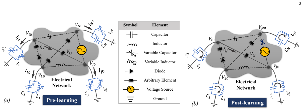
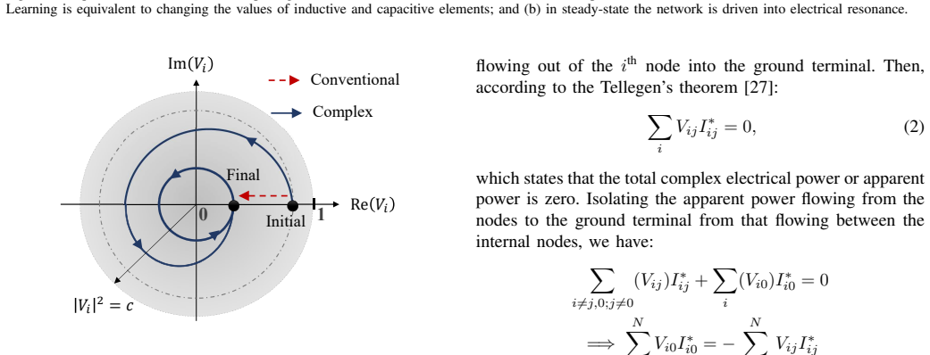
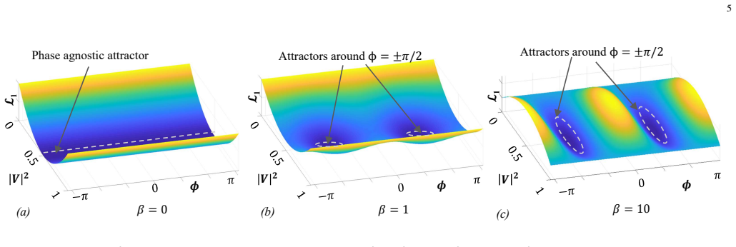
The central object is the complex growth transform dynamical system, in which each voltage evolves as $\partial V_i/\partial t = j\omega\sigma_{V_i}V_i - \Delta\sigma_{V_i}V_i$, each current evolves similarly with an added phase frequency, and the phase $\phi_i$ obeys a first-order filter $\tau_i\omega_{\phi_i} + \phi_i = g_{\phi_i}$. The load-bearing identity is Tellegen's theorem, which gives total complex power zero and lets the authors replace the zero-reactive-power constraint with conservation of reactive energy $\sum_i (\frac12 C_i|V_i|^2 + \frac12 L_i|I_i|^2) = E_0$. The phasor magnitudes carry the learning objective $H$, while the phase regularizer $\beta\sum_i |V_i|^2|I_i|^2\cos^2\phi_i$ shapes the trajectory so that steady state is reached at resonance, with $\phi_i = \pm\pi/2$ at every active node.
What would settle it
Run the update equations (15)-(18) on a two-node network from many random initial phases and record whether $\sum_i |V_i||I_i|\cos\phi_i$ converges to zero in every trial; a trajectory ending at any phase other than $\pm\pi/2$ with nonzero $|V_i||I_i|$ would disprove Theorem 1.
Extended reading notes
Core claim
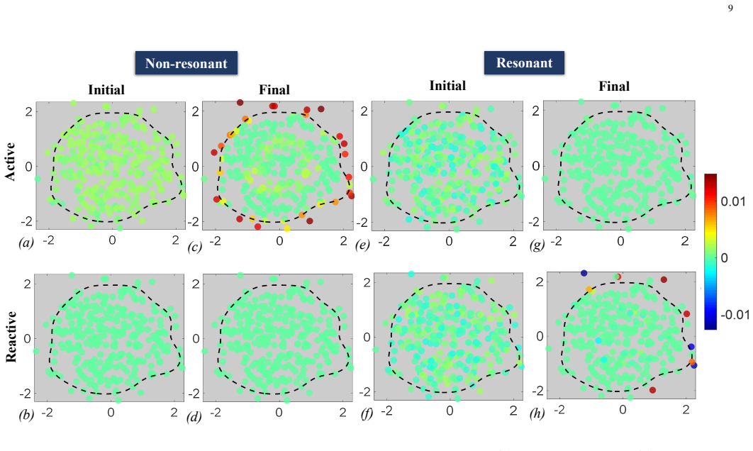
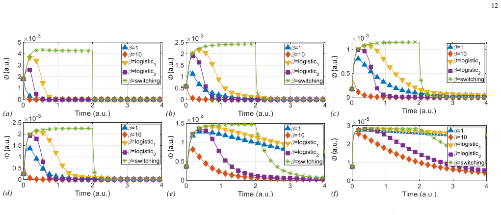
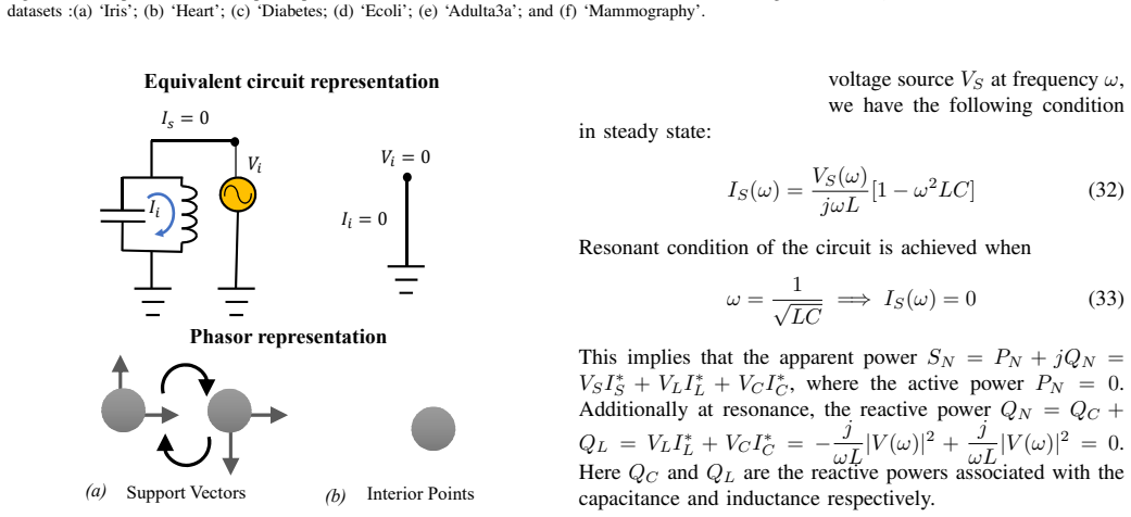
On its own terms, the paper claims that the system of nonlinear dynamical equations (15)-(18) converges to the optimal point of problem (14) in steady state. The magnitude updates follow a growth transform that monotonically decreases a Lipschitz objective, and the phase updates drive each phase angle to $\pm\pi/2$ whenever the node carries nonzero voltage and current. In steady state the active power, $\sum_i |V_i||I_i|\cos\phi_i$, is zero, so the network stores learned parameters as limit-cycle oscillations sustained by capacitive and inductive reactive energy. Applied to a one-class SVM with $\alpha_i = |V_i|^2 + |I_i|^2$, support vectors correspond to LC tanks at resonance and interior points to grounded sinks, and the resonant model is reported to dissipate less active power than the non-resonant variant.
Load-bearing premise
The zero-power conclusion rests on the assumption that the rule for adjusting the voltage-current phase always lowers the cost and always settles at a 90-degree offset; if some other phase offset can be stable, the trained network will keep dissipating power.
Editorial extensions
If this is right
- A trained one-class SVM can in principle be stored as self-sustained LC oscillations, drawing no active power from the supply in steady state.
- The annealing schedule for $\beta$ trades convergence speed against active-power dissipation during learning, allowing different operating points between fast learning and low energy use.
- The same construction applies to any learning problem of the form (26) over a probability simplex, including probabilistic models, and to coupled-oscillator networks for optimization and pattern matching.
- The network remains at resonance under a global phase shift or a relative phase shift between voltage and current, so the learned solution is invariant to common phase drifts.
- The second-order dynamics split into a conservative limit-cycle term and a dissipative term, which the paper reads as a stable limit cycle robust to small perturbations.
Reading between the lines
- If the zero-active-power steady state is robust in hardware, energy-based analog inference could run continuously on stored reactive energy, making always-on edge classifiers plausible.
- The phase variable offers a physical substrate for synchronization; a testable extension is whether the resonant SVM's support vectors phase-lock, linking classification margins to oscillator synchronization.
- A direct numerical check of the phase subsystem alone, starting from many random initial phases and recording where $\phi_i$ settles, would isolate the unproven Condition 3 without building any circuit.
- Because the learned solution lives in the frequency and phase of oscillations, perturbation recovery on the limit cycle suggests a form of analog error correction absent in dissipative energy-based models.
Signed reviews
Editorial analysis
A structured set of objections, weighed in public.
Referee Report
Summary. This manuscript proposes a complex-domain, continuous-time growth-transform dynamical system for solving constrained optimization problems whose variables are interpreted as voltage and current phasors of an electrical network. The central idea is to augment a magnitude-only objective H(|V_i|,|I_i|) with an active-power dissipation regularizer β∑|V_i|^2|I_i|^2 cos^2 φ_i and a conserved reactive-energy constraint ∑(|V_i|^2+|I_i|^2)=1. The paper states Theorem 1 claiming that the coupled magnitude-phase dynamics (15)-(18) converge to the optimum of Equation (14) and reach a steady state with zero active power, i.e., φ_i=±π/2 at every node with nonzero |V_i||I_i|. It then applies the framework to one-class SVM on synthetic and real datasets, reporting dissipation profiles and support-vector counts.
Significance. The potential significance is real if the central convergence theorem can be established. The framework offers a conceptually novel energy-based learning formulation in which learned parameters are encoded in sustained LC oscillations, active power is dissipated only transiently, and an annealing schedule trades off convergence speed against dissipation. The paper also provides a general mapping from probabilistic optimization problems to phasor magnitudes, and its simulation study covers multiple annealing schedules, random initializations, and several benchmark datasets. The writing is generally clear. However, the main theorem currently rests on an unproved Lyapunov inequality for the coupled phase-magnitude dynamics, and the physical equivalence used to motivate the conservation constraint is stated too strongly. These issues are central rather than cosmetic.
major comments (3)
- [Appendix C, Condition 3 (Eqs. (15)-(18), (57)-(59))] The proof of the phase update is asserted, not derived. The text says "We can then apply the growth transform dynamical system [7] to get" and then jumps to Eq. (57) and the resulting Eq. (17); no Lyapunov inequality is established for the coupled system in which the magnitude updates (15)-(16) depend on φ through ∂L/∂V_i and ∂L/∂I_i, and the phase update (17) depends on the magnitudes through ∂L/∂φ_i. Since the steady-state zero-active-power claim is exactly the statement that φ_i=±π/2 for every node with |V_i||I_i|≠0, this missing monotonicity argument is load-bearing for Theorem 1. Please supply the missing derivation or explicitly weaken the theorem to a conjecture supported by simulations.
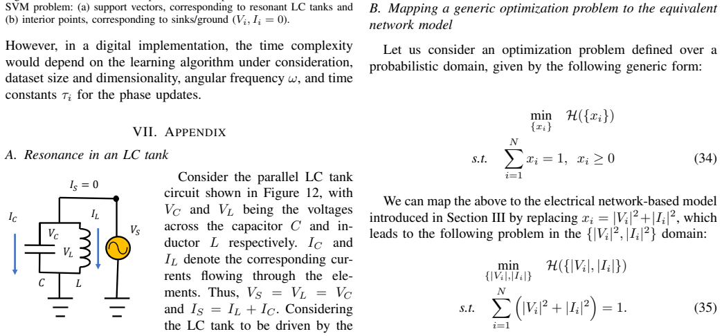
- [Section III, Eqs. (5)-(6)] The claim that zero total reactive power, ∑ [V_i(C_i dV_i/dt)* + (L_i dI_i/dt) I_i*]=0, is equivalent to conservation of reactive energy ∑(1/2 C_i|V_i|^2 + 1/2 L_i|I_i|^2)=E0 is not correct in general. In sinusoidal steady state the left side is an imaginary-power balance involving ω∑(L_i|I_i|^2 - C_i|V_i|^2), not the time derivative of the stored energy; the derivative of the stored energy is related to real power. This conflation affects the physical interpretation of the normalization constraint (9) and of the claimed electrical-resonance equivalence. The optimization can still be posed with (9) as a normalization constraint, but the stated equivalence should be corrected or qualified.
- [Appendix C, Lemma leading to Eqs. (50)-(53)] The continuous-time limit is not derived with the required rate normalization. The discrete update (52) contains the term V_{i,n-1} Δσ_{V_i,n-1}; passing to Δt→0 yields ∂V_i/∂t = jωσ_{V_i} V_i - Δσ_{V_i} V_i only if Δσ is O(Δt) (or an explicit time constant is introduced and the terms are scaled accordingly). No such normalization is specified, so the continuous-time dynamics (15)-(16) are only heuristically justified. Please provide a rigorous limiting argument or state the heuristic status of this step.
minor comments (5)
- [Table numbering, Section V] Table 2 is introduced for the growth-transform system in Section IV, and then a second Table 2 titled "Performance on real benchmark datasets" appears in Section V; the second table should be renumbered and all references updated.
- [Theorem 1 statement] The sum in the theorem statement, ∑_{n=1}^N |V_i||I_i| cos φ_i, uses index n in the summation but i in the summand; it should be ∑_{i=1}^N |V_i||I_i| cos φ_i.
- [Section III, Eq. (4) and Eq. (7)] Equation (4) defines D with |Re{V_i I_i^*}|^2 while later the same symbol is used for |V_i|^2|I_i|^2 cos^2 φ_i. Since φ_i is defined as the phase angle between V_i and I_i, these expressions agree, but the equivalence should be stated explicitly at the first occurrence.
- [Section V, Table 2] The real-data results report only counts of inliers, outliers, and support vectors, with no baseline accuracy, ROC, or AUC comparison against a standard one-class SVM; adding such a baseline would let the reader judge whether the resonant regularizer preserves decision quality.
- [Figures 6 and 8] The insets showing transient dynamics are very small; enlarging them would make the claimed convergence behavior easier to assess.
Circularity Check
Partial circularity: the zero-active-power steady state is baked into the objective via the cos²φ regularizer, and the phase-convergence proof leans on an asserted application of the authors' prior growth-transform result.
-
self definitional
[Section III, after Eq. (10), 'two important properties' bullet; Theorem 1]
"If β is slowly annealed to a sufficiently high value, then φi→π/2 under steady state for i :|Vi||Ii|⁄= 0. This implies that network achieves zero active power dissipation in steady state."
The regularizer in Eq. (10)/(14) is βΣ|V_i|^2|I_i|^2 cos²φ_i. Its global minima occur exactly where cos²φ_i = 0, i.e., φ_i = ±π/2, and at those points Σ|V_i||I_i|cosφ_i = 0 by elementary trigonometry. Thus the theorem's zero-active-power steady state is a property designed into the optimization objective, not an emergent consequence of the dynamics or of Tellegen/resonance physics. The dynamical system is claimed to converge to a minimizer of this pre-designed objective, so the zero-dissipation conclusion is an input of the problem formulation rather than an independent prediction.
-
self citation load bearing
[Appendix C, Condition 3, phase update derivation]
"We can split φi as φi =φ+i−φ−i, φ+i,φ−i>0, which implies that φ+i+φ−i=π. We can then apply the growth transform dynamical system [7] to get ... This implies that the voltage and current phasors corresponding to the i−th node in the network may be phase shifted by an additional amount φi with respect to the absolute reference."
The convergence of the phase variables is the load-bearing step for the zero-dissipation claim, and it is justified by applying the authors' own growth-transform system [7] to the decomposed phase pair. The text then asserts 'This implies' the desired steady state without deriving a Lyapunov inequality for the actual coupled system (15)-(18), where magnitude updates depend on φ and the phase update depends on magnitudes. The conclusion φ_i = ±π/2 is exactly what the phase regularizer was constructed to enforce, so the self-citation [7] is invoked to close the gap between the constructed objective and the theorem's headline physical result.
full rationale
The paper's core mathematical proposal—the complex growth-transform dynamical system (15)-(18)—is not circular in the statistical sense: no parameter is fitted to data and then renamed a prediction, and the SVM experiments are simulations of the proposed dynamics on standard benchmarks. However, the headline outcome, steady-state zero active-power dissipation, is placed into the objective by construction: Eq. (10)/(14) includes βΣ|V_i|^2|I_i|^2cos²φ_i, whose minimizers are exactly the quadrature points where Σ|V_i||I_i|cosφ_i = 0. The dynamics only need to reach that pre-designed optimum. Furthermore, the proof that the coupled system decreases L is incomplete: Appendix C, Condition 3 applies the authors' earlier growth-transform result [7] to the phase pair and then asserts the desired convergence for the full coupled magnitude-phase system; no monotonicity proof for the coupled system is supplied. This is partly a proof gap and partly a self-citation load-bearing step, but combined with the by-construction regularizer it makes the zero-dissipation claim substantially less independent than the paper's framing suggests. Overall, partial circularity with genuine independent content in the dynamical-system derivation, so a moderate score rather than a full reduction.
Assumptions & free parameters
free parameters (7)
- beta (active-power regularization weight) =
1 or 10 in experiments; logistic and switching annealing schedules
- angular frequency omega =
pi/10, pi/4, pi/20, pi/8 in experiments
- kernel width sigma =
1, 10, 20 for synthetic datasets
- nu (OC-SVM regularization) =
0.1
- lambda (growth-transform positivity constant) =
not reported
- time constants tau_i for phase updates =
not reported
- annealing hyperparameters k and t0 =
not reported numerically
assumptions (6)
- standard math Tellegen's theorem: total complex power over all network nodes is zero (Eq. 2).
- standard math Baum-Eagon inequality / growth transform convergence for Lipschitz continuous objective functions on the probability simplex.
- standard math Wirtinger calculus for derivatives of real-valued functions of complex variables.
- ad hoc to paper Zero reactive power is equivalent to conservation of total reactive energy (Eqs. 5-6).
- domain assumption The learning objective H depends only on magnitudes |V_i| and |I_i|, allowing phase angles to be controlled independently.
- domain assumption Every learning parameter alpha_i can be encoded as |V_i|^2 + |I_i|^2 with V_i and I_i independent (Eq. 27).
invented entities (2)
-
Reactive energy E0 (or its normalized version) as a conserved quantity
-
Resonant LC tank interpretation of support vectors
Cite this review
Pith. "Pith review of Resonant Machine Learning Based on Complex Growth Transform Dynamical Systems." pith.science (2026). https://pith.science/paper/WH5BX43X
@misc{pith2026190805377,
  author       = {Pith},
  title        = {Pith review of: Resonant Machine Learning Based on Complex Growth Transform Dynamical Systems},
  year         = {2026},
  howpublished = {\url{https://pith.science/paper/WH5BX43X}},
  note         = {Machine review of arXiv:1908.05377}
}
read the original abstract
Traditional energy-based learning models associate a single energy metric to each configuration of variables involved in the underlying optimization process. Such models associate the lowest energy state to the optimal configuration of variables under consideration, and are thus inherently dissipative. In this paper we propose an energy-efficient learning framework that exploits structural and functional similarities between a machine learning network and a general electrical network satisfying the Tellegen's theorem. In contrast to the standard energy-based models, the proposed formulation associates two energy components, namely, active and reactive energy to the network. This ensures that the network's active-power is dissipated only during the process of learning, whereas the reactive-power is maintained to be zero at all times. As a result, in steady-state, the learned parameters are stored and self-sustained by electrical resonance determined by the network's nodal inductances and capacitances. Based on this approach, this paper introduces three novel concepts: (a) A learning framework where the network's active-power dissipation is used as a regularization for a learning objective function that is subjected to zero total reactive-power constraint; (b) A dynamical system based on complex-domain, continuous-time growth transforms which optimizes the learning objective function and drives the network towards electrical resonance under steady-state operation; and (c) An annealing procedure that controls the trade-off between active-power dissipation and the speed of convergence. As a representative example, we show how the proposed framework can be used for designing resonant support vector machines (SVMs), where we show that the support-vectors correspond to an LC network with self-sustained oscillations.
Figures

Figures from the paper (9 more)




Reference graph
Works this paper leans on
-
[7]
Decentralized global optimization based on a growth transform dynamical system model,
O. Chatterjee and S. Chakrabartty, “Decentralized global optimization based on a growth transform dynamical system model,” IEEE Trans- actions on Neural Networks and Learning Systems , vol. 29, no. 12, pp. 6052–6061, 2018
work page 2018
-
[1]
A tutorial on energy-based learning,
Y . LeCun, S. Chopra, R. Hadsell, M. Ranzato, and F. Huang, “A tutorial on energy-based learning,” Predicting Structured Data , vol. 1, no. 0, 2006
work page 2006
-
[2]
Neural computation of decisions in optimization problems,
J. J. Hopfield and D. W. Tank, “Neural computation of decisions in optimization problems,” Biological Cybernetics, vol. 52, no. 3, pp. 141– 152, 1985
work page 1985
-
[3]
Edminister, Theory and problems of electric circuits
J. Edminister, Theory and problems of electric circuits . Schaum, 1965
work page 1965
-
[4]
M. E. V . Valkenburg, Network analysis. Prentice-Hall, 1964
work page 1964
-
[5]
Reactive power compensation technologies: State-of-the-art review,
J. Dixon, L. Moran, J. Rodriguez, and R. Domke, “Reactive power compensation technologies: State-of-the-art review,” Proceedings of the IEEE, vol. 93, no. 12, pp. 2144–2164, 2005
work page 2005
-
[6]
W. Hofmann, J. Schlabbach, and W. Just, Reactive power compensation: a practical guide . John Wiley & Sons, 2012. 15
work page 2012
-
[8]
Support vector method for novelty detection,
B. Sch ¨olkopf, R. C. Williamson, A. J. Smola, J. Shawe-Taylor, and J. C. Platt, “Support vector method for novelty detection,” in Advances in Neural Information Processing Systems , pp. 582–588, 2000
work page 2000
Show all 42 references
-
[9]
From kuramoto to crawford: exploring the onset of synchronization in populations of coupled oscillators,
S. H. Strogatz, “From kuramoto to crawford: exploring the onset of synchronization in populations of coupled oscillators,” Physica D: Nonlinear Phenomena, vol. 143, no. 1-4, pp. 1–20, 2000
2000
-
[10]
The character of physical law,
R. Feynman, “The character of physical law,” 2017
2017
-
[11]
A unified energy-based framework for unsupervised learning,
Y .-L. Boureau, S. Chopra, Y . LeCun, et al. , “A unified energy-based framework for unsupervised learning,” in Artificial Intelligence and Statistics, pp. 371–379, 2007
2007
-
[12]
Optimal perceptual inference,
G. E. Hinton and T. J. Sejnowski, “Optimal perceptual inference,” in Proceedings of the IEEE conference on Computer Vision and Pattern Recognition, pp. 448–453, 1983
1983
-
[13]
Restricted boltzmann machines for collaborative filtering,
R. Salakhutdinov, A. Mnih, and G. Hinton, “Restricted boltzmann machines for collaborative filtering,” in Proceedings of the 24th inter- national conference on Machine learning , pp. 791–798, ACM, 2007
2007
-
[14]
Equilibrium propagation: Bridging the gap between energy-based models and backpropagation,
B. Scellier and Y . Bengio, “Equilibrium propagation: Bridging the gap between energy-based models and backpropagation,” Frontiers in Computational Neuroscience, vol. 11, p. 24, 2017
2017
-
[15]
Learning deep energy models,
J. Ngiam, Z. Chen, P. W. Koh, and A. Y . Ng, “Learning deep energy models,” in Proceedings of the 28 th International Conference on Machine Learning, 2011
2011
-
[16]
Deep structured energy based models for anomaly detection,
S. Zhai, Y . Cheng, W. Lu, and Z. Zhang, “Deep structured energy based models for anomaly detection,” in International Conference on Machine Learning, pp. 1100–1109, 2016
2016
-
[17]
Reinforcement learning with deep energy-based policies,
T. Haarnoja, H. Tang, P. Abbeel, and S. Levine, “Reinforcement learning with deep energy-based policies,” in Proceedings of the 34th Interna- tional Conference on Machine Learning-Volume 70 , pp. 1352–1361, JMLR. org, 2017
2017
-
[18]
Energy-inspired models: Learning with sampler-induced distributions,
J. Lawson, G. Tucker, B. Dai, and R. Ranganath, “Energy-inspired models: Learning with sampler-induced distributions,” in Advances in Neural Information Processing Systems , pp. 8499–8511, 2019
2019
-
[19]
Hirose, Complex-valued neural networks: theories and applications , vol
A. Hirose, Complex-valued neural networks: theories and applications , vol. 5. World Scientific, 2003
2003
-
[20]
Deep complex networks,
C. Trabelsi, O. Bilaniuk, Y . Zhang, D. Serdyuk, S. Subramanian, J. F. Santos, S. Mehri, N. Rostamzadeh, Y . Bengio, and C. J. Pal, “Deep complex networks,” arXiv preprint arXiv:1705.09792 , 2017
2017 arXiv
-
[21]
Deep quaternion networks,
C. J. Gaudet and A. S. Maida, “Deep quaternion networks,” in 2018 International Joint Conference on Neural Networks (IJCNN) , pp. 1–8, IEEE, 2018
2018
-
[22]
On complex valued convolutional neural networks,
N. Guberman, “On complex valued convolutional neural networks,” arXiv preprint arXiv:1602.09046 , 2016
2016 arXiv
-
[23]
Complex support vector machines for regression and quaternary classification,
P. Bouboulis, S. Theodoridis, C. Mavroforakis, and L. Evaggelatou- Dalla, “Complex support vector machines for regression and quaternary classification,” IEEE Transactions on Neural Networks and Learning Systems, vol. 26, no. 6, pp. 1260–1274, 2014
2014
-
[24]
A mathematical motivation for complex-valued convolutional networks,
J. Bruna, S. Chintala, Y . LeCun, S. Piantino, A. Szlam, and M. Tygert, “A mathematical motivation for complex-valued convolutional networks,” arXiv preprint arXiv:1503.03438 , 2015
2015 arXiv
-
[25]
Orthogonality of decision boundaries in complex-valued neural networks,
T. Nitta, “Orthogonality of decision boundaries in complex-valued neural networks,” Neural Computation, vol. 16, no. 1, pp. 73–97, 2004
2004
-
[26]
Complex-valued restricted boltzmann machine for direct learning of frequency spectra.,
T. Nakashika, S. Takaki, and J. Yamagishi, “Complex-valued restricted boltzmann machine for direct learning of frequency spectra.,” in INTER- SPEECH, pp. 4021–4025, 2017
2017
-
[27]
A general network theorem, with applications,
B. D. Tellegen, “A general network theorem, with applications,” Philips Res Rep, vol. 7, pp. 256–269, 1952
1952
-
[28]
The elements of statistical learning: data mining, inference and prediction,
T. Hastie, R. Tibshirani, J. Friedman, and J. Franklin, “The elements of statistical learning: data mining, inference and prediction,” The Mathematical Intelligencer, vol. 27, no. 2, pp. 83–85, 2005
2005
-
[29]
K. P. Murphy, Machine learning: a probabilistic perspective. MIT press, 2012
2012
-
[30]
Probabilistic machine learning and artificial intelli- gence,
Z. Ghahramani, “Probabilistic machine learning and artificial intelli- gence,” Nature, vol. 521, no. 7553, p. 452, 2015
2015
-
[31]
Gini support vector machine: Quadratic entropy based robust multi-class probability regression,
S. Chakrabartty and G. Cauwenberghs, “Gini support vector machine: Quadratic entropy based robust multi-class probability regression,” Jour- nal of Machine Learning Research , vol. 8, no. Apr, pp. 813–839, 2007
2007
-
[32]
Support vector domain description,
D. M. Tax and R. P. Duin, “Support vector domain description,” Pattern Recognition Letters, vol. 20, no. 11-13, pp. 1191–1199, 1999
1999
-
[33]
Extended poly- nomial growth transforms for design and training of generalized support vector machines,
A. Gangopadhyay, O. Chatterjee, and S. Chakrabartty, “Extended poly- nomial growth transforms for design and training of generalized support vector machines,” IEEE Transactions on Neural Networks and Learning Systems, vol. 29, no. 5, pp. 1961–1974, 2017
1961
-
[34]
UCI machine learning repository
D. Dua and C. Graff, “UCI machine learning repository.” http://archive. ics.uci.edu/ml, 2017
2017
-
[35]
ODDS library
S. Rayana, “ODDS library.” http://odds.cs.stonybrook.edu, 2016
2016
-
[36]
Computing with networks of oscillatory dynamical systems,
A. Raychowdhury, A. Parihar, G. H. Smith, V . Narayanan, G. Csaba, M. Jerry, W. Porod, and S. Datta, “Computing with networks of oscillatory dynamical systems,”Proceedings of the IEEE, vol. 107, no. 1, pp. 73–89, 2019
2019
-
[37]
Neuromorphic computing with nanoscale spintronic oscillators,
J. Torrejon, M. Riou, F. A. Araujo, S. Tsunegi, G. Khalsa, D. Querlioz, P. Bortolotti, V . Cros, K. Yakushiji, A. Fukushima,et al., “Neuromorphic computing with nanoscale spintronic oscillators,” Nature, vol. 547, no. 7664, p. 428, 2017
2017
-
[38]
M. A. Nielsen and I. L. Chuang, Quantum computation and quantum information. Cambridge university press, 2010
2010
-
[39]
Continuous- time optimization using sub-threshold current-mode growth transform circuits,
A. Gangopadhyay, O. Chatterjee, and S. Chakrabartty, “Continuous- time optimization using sub-threshold current-mode growth transform circuits,” in 2018 IEEE 61st International Midwest Symposium on Circuits and Systems (MWSCAS) , pp. 246–249, IEEE, 2018
2018
-
[40]
Growth transformations for functions on manifolds,
L. E. Baum and G. Sell, “Growth transformations for functions on manifolds,” Pacific Journal of Mathematics , vol. 27, no. 2, pp. 211– 227, 1968
1968
-
[41]
A generalization of the baum algorithm to rational objective functions,
P. Gopalakrishnan, D. Kanevsky, A. Nadas, and D. Nahamoo, “A generalization of the baum algorithm to rational objective functions,” in International Conference on Acoustics, Speech, and Signal Processing , pp. 631–634, IEEE, 1989
1989
-
[42]
Wirtinger calculus based gradient descent and levenberg-marquardt learning algorithms in complex-valued neural networks,
M. F. Amin, M. I. Amin, A. Y . H. Al-Nuaimi, and K. Murase, “Wirtinger calculus based gradient descent and levenberg-marquardt learning algorithms in complex-valued neural networks,” inInternational Conference on Neural Information Processing , pp. 550–559, Springer, 2011
2011
Reviewed August 14, 2026 · model on record in the stance chip above.
Discussion (0). Continue with ORCID to comment.