Residual Force Polytope: Admissible Task-Space Forces of Dynamic Trajectories

Carlo Tiseo; Henrique Ferrolho; Sethu Vijayakumar; Wolfgang Merkt

REVIEW 3 major objections 4 minor 31 references

Residual Force Polytope: Admissible Task-Space Forces of Dynamic Trajectories

T0 review · 3 major / 4 minor · reviewed 2026-08-14 · deepseek-v4-flash

Challenge this review Re-run · record.json Download PDF Read on arXiv ↗ Review JSON

Pith's one-line read Optimizing trajectories over the residual force polytope yields motions that withstand larger unknown disturbances than standard objectives.

desk verdict A useful dynamic-aware force polytope idea, but the redundant-arm construction over-approximates the true admissible-force set and is used as both the objective and the evaluation metric, so the central robustness claim is not yet supported. read the letter →

arxiv 1908.05380 v3 pith:D4737R25 submitted 2019-08-15 cs.RO

Henrique Ferrolho , Wolfgang Merkt , Carlo Tiseo , Sethu Vijayakumar This is my paper · ORCID

classification cs.RO

keywords residualforcepolytoperobustnesstrajectoryoptimizationpolytopestask-spaceforcesmanipulabilityroboticarms

verification ladder T0 review T1 audit T2 compute T3 formal

The pith

A machine-rendered reading of the paper's core claim, the machinery that carries it, and where it could break.

The reading

The paper introduces the residual force polytope, an exact convex representation of the task-space forces a robot can still exert or resist at any instant of a dynamic trajectory without abandoning its planned motion: the set of forces reachable from the joint torques left over after the nominal torques of the motion are subtracted from the actuation limits, mapped through the inverse-transpose Jacobian $J_e^{-\top}$ to the end-effector frame. Its central claim is that an optimization objective built from this polytope—maximizing the radius of the largest ball, centered at the end-effector, that fits inside it—produces trajectories that are more robust to unknown external disturbances than objectives based on torque minimization, manipulability maximization, or the classical quasi-static force polytope. The authors demonstrate this on a 7-DoF arm, where the residual-polytope objective beat all alternatives in admissible disturbance force over the whole trajectory, and they report that the cost of polytope operations restricts the method to offline planning for now.

What carries the argument

The residual force polytope $P'(q,\tau)$: the convex polytope of task-space forces obtained by mapping the torque margin $\tau_{\text{lim}} - \tau$, i.e., the nominal torques of the motion subtracted from the joint actuation limits, through the inverse-transpose Jacobian $J_e^{-\top}$ into the end-effector frame. It is the exact, dynamics-aware replacement for the quasi-static force polytope: because the nominal torques of each trajectory point are decision variables in the direct transcription, an objective built from $P'$ cannot merely inflate geometric manipulability but must preserve torque authority against the very motion being demanded. Two metric computations carry the evaluation. The first is the inscribed-ball radius, solved as the linear program that maximizes $r$ subject to $B(0,r) \subseteq P'$ with the ball center fixed at the end-effector origin, which measures isotropic robustness to forces from unknown directions. The second is the volume of the intersection $P' \cap C$ with an uncertainty cone $C$, which measures robustness to forces from a roughly known direction. The double-description method for converting between half-space and vertex representations drives the computational cost, which the paper measures at roughly 22–24 $\mu$s per polytope construction but 6.3–7.4 ms per ball, intersection, or volume operation, and which restricts the objectives to offline planning.

What would settle it

Run a $g_E$-optimized trajectory and a torque-minimized ($g_A$) trajectory on the same robot, or in a simulation with a tracking controller, friction, and measurement noise, and apply an external force impulse of increasing magnitude from random directions to the end-effector, recording the largest impulse each motion rejects before torque saturation or a set tracking-error bound is exceeded; if the $g_A$ trajectory rejects as much as the $g_E$ trajectory despite its smaller inscribed-ball radii, the residual force polytope does not predict real robustness. A minimal check: compare the metric's predicted admissible force at a single trajectory point against the largest push the closed-loop system actually tolerates at that point.

Watch

Extended reading notes

Core claim

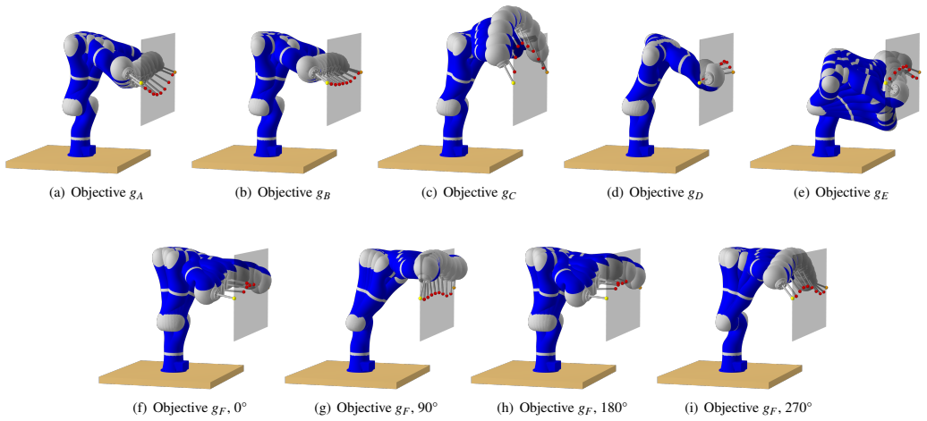
The paper's central object is the residual force polytope $P'(q,\tau)$: given the equations of motion $M(q)\dot v + h(q,v) = \tau + J_e^\top(q) f_{\text{tip}}$, the residual torques $\tau_{\text{lim}} - \tau_{\text{nominal}}$ are mapped through $f_{\text{tip}} = J_e^{-\top}\tau_{f_{\text{tip}}}$ to obtain the convex set of end-effector forces that can be resisted without saturating any joint and without interfering with the nominal motion. From this object the paper extracts two scalar robustness metrics: the radius of the largest ball centered at the end-effector inscribed in the polytope—a linear program, i.e., a Chebyshev-center problem with the ball center fixed—for disturbances of unknown direction, and the volume of the polytope's intersection with a cone aligned to an expected force direction, for partially known disturbances. Both metrics are summed over all mesh points as objectives $g_E$ and $g_F$ in a direct-transcription optimal control problem for a 7-DoF KUKA LWR arm, alongside comparison objectives $g_A$–$g_D$ (torque minimization, residual-torque maximization, manipulability maximization, and the quasi-static force-polytope inscribed ball). The paper's central result, reported for both interior-point and active-set solvers, is that $g_E$ yields trajectories with greater admissible force magnitude over the entire trajectory than every alternative, improving on $g_D$ by $53.2\pm6.52$ N without payload and $40.55\pm21.37$ N with a 2 kg payload, while the cone-based $g_F$ gives still larger margins when the disturbance direction is correctly anticipated but saturates the actuators when the disturbance arrives from the opposite direction.

Load-bearing premise

The load-bearing premise is that the radius of the largest ball of end-effector forces that fits inside the residual force polytope is what real robustness to unknown disturbances consists of; the experiments test that radius only on the planned open-loop trajectories, with no feedback controller, hardware, friction, or sensor noise in the loop, so if that geometric radius does not predict how the closed-loop robot actually rejects disturbances, the comparison that supports the central claim collapses.

Editorial extensions

If this is right

Trajectories optimized with $g_E$, the sum of inscribed-ball radii in residual force polytopes, have greater admissible force against disturbances from any direction over the whole trajectory than trajectories from $g_A$–$g_D$, under both interior-point and active-set solvers, so robustness can be put into the plan rather than left to the controller.
Using the residual force polytope instead of the quasi-static force polytope in the same objective adds $53.2\pm6.52$ N of admissible force without payload and $40.55\pm21.37$ N with a 2 kg payload for the tested 1 s trajectories, showing that the static polytope overestimates the capability actually available while a motion is running.
Direction-specialized plans ($g_F$) beat isotropic plans ($g_E$) in margin when the disturbance comes as predicted, but saturate joint torques when it comes from the opposite direction, so isotropic planning is the safer default unless the disturbance direction is nearly certain.
The residual force polytope can be computed once per mesh point for any given trajectory, which makes it an offline evaluation tool for ranking arbitrary motions by robustness even when no optimization is involved.
The extra cost of the residual variant over the static one is small; the expensive operations are the polytope geometry routines themselves, so the paper's sketched remedies—evaluating the polytope less often or approximating its geometry—are the concrete routes toward online use.

Reading between the lines

Editorial extensions of the paper, not claims the author makes directly.

The paper validates its metric only on open-loop trajectories, so the natural unrun experiment is a closed-loop one: whether the inscribed-ball radius predicts realized disturbance rejection under a feedback controller with friction, noise, and tracking error is an open question, and the central claim's practical value hinges on it.
The cone model implies a continuum of specialization: any estimated distribution of disturbance directions—from contact geometry, terrain statistics, or prior trials—could be encoded in the cone's axis and aperture, letting a planner interpolate between the isotropic objective $g_E$ and the fully specialized $g_F$.
Because $P'(q,\tau)$ encodes actuation limits, dynamics, and the task in one covariant set, the same metric could serve system co-design (e.g., actuator sizing or mounting-choice selection) by ranking hardware according to the worst-case force it can resist while executing a nominal motion—an application the paper names but does not demonstrate.
A surrogate model that approximates the residual polytope geometry would settle the scalability question: if an approximate polytope preserves the robustness ranking of $g_E$ over $g_A$–$g_D$ while cutting evaluation time from milliseconds to microseconds, the approach could move from offline to near-online planning.

Share X Bluesky LinkedIn Reddit HN

Signed reviews

No signed human review yet.

Editorial analysis

A structured set of objections, weighed in public.

Desk editor's note, referee report, and a circularity audit.

Desk Editor's Note

read the letter

Two things to know upfront. First, the idea is genuinely new and useful: subtract the nominal torque trajectory from the actuation limits and map the remainder to task space, giving a dynamic-aware robustness measure that connects trajectory optimization to disturbance rejection. Second, the way they build that mapping for a redundant arm is mathematically wrong, and because the same object is both the cost and the evaluation metric, the main empirical claim doesn't yet stand.

What's good: the paper is clear and honest. The residual force polytope (Sec. 4) and the two uncertainty models (ball, cone) are well motivated. The experiments compare six objectives under two NLP solvers, with and without payload, and the computational-cost breakdown is refreshingly candid. The admitted limits on scalability are accurate, and the related work is fair.

Now the soft spots. The stress-test you sent is right. For the KUKA arm, n=7 and the task space is 3D linear forces, so J^T is rectangular. The correct set of end-effector forces consistent with the residual torque box is Q = {f : τ_nom + J^T f ∈ [τ_lb, τ_ub]}, an H-polyhedron in R^m. The paper instead maps the residual torque box through (J^T)^+ and calls the image exact. For non-square J, that image is generally a strict superset of Q: a torque with a null-space component projects to a smaller torque, and the corresponding force can require a torque outside the box. So the 'exact representation' claim in the Introduction and Conclusions is false. This matters doubly because gE maximizes the Chebyshev-ball radius of this over-approximated set, and Section 7.2 evaluates all trajectories with the same radius on the same over-approximated set. Figure 7's ranking of gE first is therefore circular, or at least not probative for true robustness. The impulse test in 7.3 is meant to be independent, but it says it computes required torques 'with equation (2)', which maps torque to force; the correct map from an external force to torque is τ = J^T f. If they used the pseudo-inverse in the wrong direction, that test is also invalid.

What still holds: the conceptual move—account for the nominal motion's torque demand when measuring remaining capability—is sound and can be repaired by defining the residual force polytope as the H-rep set Q, or by acknowledging the over-approximation and validating against the exact set. The comparison framework (gA–gF, payload, solver choice) is a solid template for revision.

Bottom line: the paper deserves serious peer review but not in its current form. I'd send it to referees expecting major revision, and the pseudoinverse issue must be resolved or openly scoped before publication. Don't cite it yet as a correct method. It would make a good reading-group discussion about polytope mappings and evaluation circularity.

Referee Report

3 major / 4 minor

Summary. This paper introduces the residual force polytope, defined as the image under the (pseudo)inverse of the end-effector Jacobian transpose of the box of joint torques remaining after subtracting the nominal torques of a planned trajectory. It uses the Chebyshev-ball radius of this polytope as an isotropic robustness metric, a cone-intersection volume as a directional robustness metric, and embeds both as objective functions in a direct-transcription trajectory optimization for a 7-DoF KUKA arm. The experiments compare objectives gA-gF, report that gE (residual force polytope radius) yields trajectories with larger admissible force magnitudes, benchmark interior-point versus SQP methods, and test directional robustness of gE versus gF under a synthetic impulse.

Significance. If the representation were exact and the evaluation independent, this would be a useful offline planning and design tool: it replaces ellipsoidal manipulability approximations with a convex polytope that respects actuation limits, accounts for the torques required by the motion, and yields interpretable margin metrics. The paper is clearly written, the polytope/LP machinery is standard, and the computational benchmarks in Tables 1-4 are a useful practical contribution. However, the headline claim is currently supported only by evaluating trajectories with the same quantity that objective gE maximizes, and the polytope construction itself over-approximates the true admissible-force set for a redundant arm. These issues must be resolved before the robustness claim can be accepted.

major comments (3)

[Section 3.2, Eq. (2); Section 4] For the redundant case n > m considered in the experiments, the residual force polytope P'_F = (J_e^T)^+ P'_tau is not equal to the true set Q = { f in R^m : tau_lb <= tau_nom + J_e(q)^T f <= tau_ub }. The pseudoinverse discards the component of each residual torque orthogonal to range(J_e^T), and a force is in the pseudo-inverse image exactly when the projection of the residual torque onto range(J_e^T) lies in the residual torque box. This condition is weaker than requiring J_e(q)^T f itself to lie in the box, because the projection of a box onto a subspace can be strictly larger than the intersection of the box with that subspace. Hence P'_F can contain forces whose induced joint torques violate the actuation limits, contradicting the 'exact representation' claimed in the Conclusions and the claim in Section 2 that the approach determines 'the exact margins remaining before torque saturation occurs.' This over-approximation affects both objective gE and the evaluation metric in Section 7.2.
[Section 7.2 and Eq. (18)] The evaluation metric used to rank trajectories is identical to the objective being optimized. Equation (18) defines gE as the sum over mesh points of Br(P'_k), the radius of the largest ball centered at the end-effector and inscribed in the residual force polytope, and Section 7.2 states that each trajectory is evaluated by computing the same residual force polytope and taking the same largest inscribed ball radius. Consequently, Figure 7 demonstrates that maximizing a function improves that same function, which is a tautological comparison unless Br(P') is independently shown to predict closed-loop robustness to unknown external disturbances. The impulse test in Section 7.3 does not provide that independent validation: it compares only gE with gF, and it computes the required extra torques using Eq. (2), the same pseudoinverse mapping that defines the polytope. The paper should add an evaluation against the exact admissible set, a closed-loop simulation, or a hardware experiment.
[Sections 7.3 and 8.1] The paper motivates robustness by sensor noise, signal delay, and model mismatches, but the experimental validation contains no feedback controller, no friction or noise model, and no hardware data. The planned torque margins are evaluated open-loop, so the central claim that the resulting trajectories are 'more robust to unknown external disturbances' is not independently supported. At minimum, a closed-loop torque-control simulation with a disturbance observer or a hardware disturbance-rejection test should be reported; Section 8.1's discussion of scalability does not substitute for such validation.

minor comments (4)

[Eq. (15)] The notation tau_lim in Eq. (15) is ambiguous: Eq. (3) defines per-joint scalar limits, so the objective should state explicitly whether tau_lim is a vector of per-joint limits and how asymmetric bounds are handled.
[Section 3.2, Eq. (2)] The symbol J_e^{-T} suggests invertibility, but for n > m the object used is the Moore-Penrose pseudoinverse; please write (J_e^T)^+ consistently and state the rank assumption needed for the pseudoinverse formula.
[Section 5.1] The LP for the largest inscribed ball should state explicitly that the polytope is expressed in the end-effector frame and that the ball center is the origin of that frame; the phrase 'centered at the end-effector' is correct but less precise.
[Figure 7] The caption says the plots show objectives gA-gE, while Figure 5 includes panels for gF; consider clarifying that gF is omitted because it is direction-dependent and treated separately in Section 7.3.

Circularity Check

1 steps flagged · score 6.0 of 10

Central comparison is circular: gE maximizes exactly the Chebyshev-ball radius Br(P′_k) that Section 7.2 uses as the robustness evaluation metric, so Figure 7's ranking is by construction; only the impulse test in Section 7.3 is partially independent.

fitted input called prediction [Section 6.3, Eq. (18); Section 7.2 (Robustness to External Disturbances)]
"gE : max_ξ Σ_{k=1}^M Br(P′_k) (18) ... where Br(·) denotes the radius of the largest ball centered at the end-effector and inscribed in the given polytope. ... we define our evaluation metric as the magnitude of the maximum admissible force considering all possible force directions. Therefore, each trajectory is evaluated as follows: for each point, (i) compute the residual force polytope, then (ii) find the largest ball centered at the end-effector inscribed in that polytope, and (iii) take the radius of the ball as the robustness metric. This is how we computed the forces shown in Figure 7."

Objective gE maximizes the sum over mesh points of Br(P′_k), the Chebyshev-ball radius of the residual force polytope. Section 7.2 evaluates 'robustness to external disturbances' by computing, at each point, the same Br(P′_k) and plotting its magnitude over time (Figure 7). Thus the statement that 'the trajectory computed with the residual force polytope resulted in greater robustness than any other objective function considered' is a comparison in which gE optimized the exact scalar being measured, while gA–gD were not optimized for this quantity. The paper even notes it cares about 'robustness overall during the trajectory (area under the curve)', which matches the sum in Eq. (18).

full rationale

Score 6: The main quantitative evidence for the headline claim is circular in the specific sense that the evaluation metric in Section 7.2 is the same function that objective gE was designed to maximize (Eq. 18). For every other objective, Figure 7 measures a quantity they do not optimize, while for gE it measures exactly the optimized objective; hence the observed ranking is essentially by construction. I did not find load-bearing self-citation: [6] and other prior work are used as background, not to justify the core derivation. The residual-force-polytope construction itself is original and independently specified, and the impulse experiment in Section 7.3 provides a partially independent, direction-specific check using torque limits rather than the Chebyshev radius. No closed-loop controller or hardware experiment is reported, so the external validity of Br(P′) as a proxy for real robustness is asserted rather than demonstrated; that is a validation gap rather than a circularity by itself. The paper also claims an 'exact representation' despite using a Moore-Penrose pseudoinverse in Eq. (2) for n > m, which is a mathematical over-approximation concern rather than a circularity, and is not counted in the score. Overall: partial circularity of the central evaluation, partially redeemed by Section 7.3, giving 6/10.

Assumptions & free parameters 0 free parameters · 4 assumptions · 1 invented entities

The representation depends on standard polytope machinery and rigid-body dynamics. No free parameters are fitted to data: the numeric choices such as N=10 mesh segments, a 1 second horizon, and a 2 kg payload are experimental settings, not fitted constants. The main new construction, the residual force polytope, is a definitional object rather than an empirically constrained entity.

assumptions (4)

domain assumption The robot is a fully actuated, fixed-base rigid manipulator whose dynamics are exactly given by M(q) v_dot + h(q,v) = tau + J_e^T f_tip.
Equation (1) is stated as the system model and all trajectory optimization and robustness results inherit this assumption; no friction, flexibility, or unmodeled effects are included.
domain assumption The set of achievable end-effector forces is obtained by mapping the joint torque box through the Moore-Penrose pseudoinverse of J_e^T.
Equation (2) and Section 3.3 rely on this mapping for redundant manipulators; the pseudoinverse image is assumed to characterize the force polytope, which is nontrivial when n > m.
domain assumption The residual torque capacity after a nominal trajectory is the symmetric box (tau_lim - |tau|), and every vector in that box can be allocated to disturbance rejection independently of the nominal trajectory.
This defines the residual force polytope in Section 4; it assumes no coupling between disturbance response and the nominal tracking control, and that nominal torques are known exactly.
domain assumption External disturbances are modeled as static forces at the end-effector with isotropic (ball) or conic directional uncertainty.
Sections 5.1 and 5.2 build both the objectives and the evaluation on these disturbance models, excluding impacts, forces at other links, and contact dynamics.

invented entities (1)

Residual force polytope
purpose: Represent all end-effector forces a robot can resist while tracking a nominal dynamic trajectory, after accounting for the torques required by the motion.
This is a definitional mathematical construction obtained by shifting the joint torque box by the nominal torques and mapping through J_e^{-T}. It makes no falsifiable prediction outside the paper's own metrics, so there is no independent evidence for it as an empirical entity.

how reviews work

0 comments

Cite this review

Pith. "Pith review of Residual Force Polytope: Admissible Task-Space Forces of Dynamic Trajectories." pith.science (2026). https://pith.science/paper/D4737R25

@misc{pith2026190805380,
  author       = {Pith},
  title        = {Pith review of: Residual Force Polytope: Admissible Task-Space Forces of Dynamic Trajectories},
  year         = {2026},
  howpublished = {\url{https://pith.science/paper/D4737R25}},
  note         = {Machine review of arXiv:1908.05380}
}

read the original abstract

We propose a representation for the set of forces a robot can counteract using full system dynamics: the residual force polytope. Given the nominal torques required by a dynamic motion, this representation models the forces which can be sustained without interfering with that motion. The residual force polytope can be used to analyze and compare the set of admissible forces of different trajectories, but it can also be used to define metrics for solving optimization problems, such as in trajectory optimization or system design. We demonstrate how such a metric can be applied to trajectory optimization and compare it against other objective functions typically used. Our results show that the trajectories computed by optimizing objectives defined as functions of the residual force polytope are more robust to unknown external disturbances. The computational cost of these metrics is relatively high and not compatible with the short planning times required by online methods, but they are acceptable for planning motions offline.

Figures

Figures reproduced from arXiv: 1908.05380 by the authors.

**Figure 2.** Equation (2) transforms actuation-space representations (on the left) [PITH_FULL_IMAGE:figures/full_fig_p003_2.png] view at source ↗

**Figure 3.** Illustration of two different levels of uncertainty concerning the direction of interaction forces for two real-world scenarios. On the left, factors such as controller tracking errors or noisy state estimation can ultimately lead to inaccurate foot placement, which in turn, and depending on the terrain, can induce forces applied in unexpected directions (high direction uncertainty). In contrast, on the right, the f… view at source ↗

Figures from the paper (7 more)

**Figure 4.** Figure 4: Two distinct models for representing force disturbances: the ball [PITH_FULL_IMAGE:figures/full_fig_p004_4.png]

**Figure 5.** Figure 5: Visualization of the trajectories obtained using the interior-point method without a payload. The configuration samples are equally spaced in time. The [PITH_FULL_IMAGE:figures/full_fig_p007_5.png]

**Figure 6.** Figure 6: These plots show, for each function gA–gF, the evolution of the objective value and the feasibility error along the solver iterations. In the feasibility plots, the faint-green line at y = 10−3 denotes the absolute tolerance under which a problem is considered feasible…

**Figure 9.** Figure 9: In order to compare optimal resistance to forces from any given direction (gE) against optimal resistance to forces from a specific direction (gF), we compute the torque required by the optimized trajectories for a test impulse that matches the direction estimation us…

**Figure 7.** Figure 7: These plots show the maximum admissible force magnitudes over time of trajectories computed using objective functions [PITH_FULL_IMAGE:figures/full_fig_p009_7.png]

**Figure 8.** Figure 8: These plots show the magnitude of forces applied to the end-e [PITH_FULL_IMAGE:figures/full_fig_p009_8.png]

**Figure 10.** Figure 10: Joint torques required to complete the planned task and resist the [PITH_FULL_IMAGE:figures/full_fig_p009_10.png]

Discussion (0). Continue with ORCID to comment.

Reference graph

Works this paper leans on

31 extracted references · 29 canonical work pages

[1]

Del Prete, N

A. Del Prete, N. Mansard, Addressing Constraint Robustness to Torque Errors in Task-Space Inverse Dynamics, in: Robotics, Sciences and Sys- tems (RSS), Rome, Italy, 2015. 6Not to be confused with approximations to dynamic quantities of the con- trolled system, which our proposed representation is trying to avoid

work page 2015
[2]

Plooij, W

M. Plooij, W. Wolfslag, M. Wisse, Robust feedforward control of robotic arms with friction model uncertainty, Robotics and Autonomous Systems 70 (2015) 83 – 91

work page 2015
[3]

Xin, H.-C

G. Xin, H.-C. Lin, J. Smith, O. Cebe, M. Mistry, A Model-Based Hierar- chical Controller for Legged Systems Subject to External Disturbances, in: IEEE International Conference on Robotics and Automation (ICRA), 2018, pp. 4375–4382

work page 2018
[4]

Orsolino, M

R. Orsolino, M. Focchi, C. Mastalli, H. Dai, D. G. Caldwell, C. Sem- ini, Application of Wrench-Based Feasibility Analysis to the Online Tra- jectory Optimization of Legged Robots, IEEE Robotics and Automation Letters 3 (4) (2018) 3363–3370

work page 2018
[5]

Manchester, S

Z. Manchester, S. Kuindersma, DIRTREL: Robust Nonlinear Direct Tran- scription with Ellipsoidal Disturbances and LQR Feedback, in: Robotics, Sciences and Systems (RSS), 2017

work page 2017
[6]

Ferrolho, W

H. Ferrolho, W. Merkt, Y . Yang, V . Ivan, S. Vijayakumar, Whole-Body End-Pose Planning for Legged Robots on Inclined Support Surfaces in Complex Environments, in: IEEE-RAS 18th International Conference on Humanoid Robots (Humanoids), 2018, pp. 944–951

work page 2018
[7]

Yoshikawa, Manipulability of Robotic Mechanisms, The International Journal of Robotics Research (IJRR) 4 (2) (1985)

T. Yoshikawa, Manipulability of Robotic Mechanisms, The International Journal of Robotics Research (IJRR) 4 (2) (1985)

work page 1985
[8]

Jaquier, L

N. Jaquier, L. D. Rozo, D. G. Caldwell, S. Calinon, Geometry-aware Tracking of Manipulability Ellipsoids, in: Proceedings of Robotics: Sci- ence and Systems, Pittsburgh, Pennsylvania, 2018

work page 2018

Show all 31 references

[9]

Haviland, P

J. Haviland, P. Corke, Maximising Manipulability During Resolved-Rate Motion Control, arXiv e-prints arXiv:2002.11901 (Feb. 2020)

2002 arXiv
[10]

X. Chu, Q. Hu, J. Zhang, Path Planning and Collision Avoidance for a Multi-Arm Space Maneuverable Robot, IEEE Transactions on Aerospace and Electronic Systems 54 (1) (2018) 217–232

2018
[11]

Audren, A

H. Audren, A. Kheddar, 3D Robust Stability Polyhedron in Multicontact, IEEE Transactions on Robotics (T-RO) (2018)

2018
[12]

Hirukawa, S

H. Hirukawa, S. Hattori, K. Harada, S. Kajita, K. Kaneko, F. Kanehiro, K. Fujiwara, M. Morisawa, A Universal Stability Criterion of the Foot Contact of Legged Robots - Adios ZMP, in: IEEE International Confer- ence on Robotics and Automation (ICRA), 2006

2006
[13]

Ben-Tal, A

A. Ben-Tal, A. Nemirovski, Robust Truss Topology Design via Semidef- inite Programming, SIAM Journal on Optimization 7 (4) (1997) 991– 1016

1997
[14]

G. M. Ziegler, Lectures on polytopes, V ol. 152, Springer Science & Busi- ness Media, 2012

2012
[15]

Fukuda, A

K. Fukuda, A. Prodon, Double Description Method Revisited, in: Com- binatorics and Computer Science (CCS), Springer, 1995

1995
[16]

Chiacchio, Y

P. Chiacchio, Y . Bouﬀard-Vercelli, F. Pierrot, Force Polytope and Force Ellipsoid for Redundant Manipulators, Journal of Robotic Systems 14 (8) (1997) 613–620

1997
[17]

S. Boyd, L. Vandenberghe, Convex optimization, Cambridge university press, 2004

2004
[18]

J. T. Betts, Practical Methods for Optimal Control and Estimation Using Nonlinear Programming, 2nd Edition, V ol. 19, Society for Industrial and Applied Mathematics (SIAM), 2010

2010
[19]

von Stryk, R

O. von Stryk, R. Bulirsch, Direct and Indirect Methods for Trajectory Optimization, Annals of Operations Research (1992)

1992
[20]

Mayne, A Second-order Gradient Method for Determining Optimal Trajectories of Non-linear Discrete-time Systems, International Journal of Control 3 (1) (1966) 85–95

D. Mayne, A Second-order Gradient Method for Determining Optimal Trajectories of Non-linear Discrete-time Systems, International Journal of Control 3 (1) (1966) 85–95

1966
[21]

Tassa, N

Y . Tassa, N. Mansard, E. Todorov, Control-limited di ﬀerential dynamic programming, in: IEEE International Conference on Robotics and Au- tomation (ICRA), 2014, pp. 1168–1175

2014
[22]

Giftthaler, M

M. Giftthaler, M. Neunert, M. St ¨auble, J. Buchli, M. Diehl, A Family of Iterative Gauss-Newton Shooting Methods for Nonlinear Optimal Con- trol, in: IEEE /RSJ International Conference on Intelligent Robots and Systems, 2018

2018
[23]

Mastalli, R

C. Mastalli, R. Budhiraja, W. Merkt, G. Saurel, B. Hammoud, M. Naveau, J. Carpentier, L. Righetti, S. Vijayakumar, N. Mansard, Crocoddyl: An Eﬃcient and Versatile Framework for Multi-Contact Optimal Control, in: IEEE International Conference on Robotics and Automation (ICRA), 2020

2020
[24]

Bezanson, A

J. Bezanson, A. Edelman, S. Karpinski, V . B. Shah, Julia: A Fresh Ap- proach to Numerical Computing, SIAM Review 59 (1) (2017) 65–98

2017
[25]

R. H. Byrd, J. Nocedal, R. A. Waltz, Knitro: An Integrated Package for Nonlinear Optimization, Springer US, 2006

2006
[26]

Stouraitis, I

T. Stouraitis, I. Chatzinikolaidis, M. Gienger, S. Vijayakumar, Dyadic 11 collaborative Manipulation through Hybrid Trajectory Optimization, in: Proceedings of The 2nd Conference on Robot Learning (CoRL), V ol. 87, PMLR, 2018, pp. 869–878

2018
[27]

A. W. Winkler, C. D. Bellicoso, M. Hutter, J. Buchli, Gait and Trajectory Optimization for Legged Systems Through Phase-Based End-E ﬀector Parameterization, IEEE Robotics and Automation Letters (RA-L) 3 (3) (2018) 1560–1567

2018
[28]

M. Posa, C. Cantu, R. Tedrake, A Direct Method for Trajectory Opti- mization of Rigid Bodies Through Contact, The International Journal of Robotics Research (IJRR) 33 (1) (2014) 69–81

2014
[29]

A. W. Winkler, Optimization-based motion planning for legged robots, Ph.D. thesis, ETH Zurich, Zurich (2018)

2018
[30]

Bratta, R

A. Bratta, R. Orsolino, M. Focchi, V . Barasuol, G. G. Muscolo, C. Sem- ini, On the Hardware Feasibility of Nonlinear Trajectory Optimization for Legged Locomotion based on a Simpliﬁed Dynamics, in: IEEE Interna- tional Conference on Robotics and Automation (ICRA), 2020

2020
[31]

J. Zhen, D. den Hertog, Computing the Maximum V olume Inscribed El- lipsoid of a Polytopic Projection, INFORMS Journal on Computing 30 (1) (2018) 31–42. 12

2018

Pith tools

Reviewed August 14, 2026 · model on record in the stance chip above.

[1] [1]

Del Prete, N

A. Del Prete, N. Mansard, Addressing Constraint Robustness to Torque Errors in Task-Space Inverse Dynamics, in: Robotics, Sciences and Sys- tems (RSS), Rome, Italy, 2015. 6Not to be confused with approximations to dynamic quantities of the con- trolled system, which our proposed representation is trying to avoid

work page 2015

[2] [2]

Plooij, W

M. Plooij, W. Wolfslag, M. Wisse, Robust feedforward control of robotic arms with friction model uncertainty, Robotics and Autonomous Systems 70 (2015) 83 – 91

work page 2015

[3] [3]

Xin, H.-C

G. Xin, H.-C. Lin, J. Smith, O. Cebe, M. Mistry, A Model-Based Hierar- chical Controller for Legged Systems Subject to External Disturbances, in: IEEE International Conference on Robotics and Automation (ICRA), 2018, pp. 4375–4382

work page 2018

[4] [4]

Orsolino, M

R. Orsolino, M. Focchi, C. Mastalli, H. Dai, D. G. Caldwell, C. Sem- ini, Application of Wrench-Based Feasibility Analysis to the Online Tra- jectory Optimization of Legged Robots, IEEE Robotics and Automation Letters 3 (4) (2018) 3363–3370

work page 2018

[5] [5]

Manchester, S

Z. Manchester, S. Kuindersma, DIRTREL: Robust Nonlinear Direct Tran- scription with Ellipsoidal Disturbances and LQR Feedback, in: Robotics, Sciences and Systems (RSS), 2017

work page 2017

[6] [6]

Ferrolho, W

H. Ferrolho, W. Merkt, Y . Yang, V . Ivan, S. Vijayakumar, Whole-Body End-Pose Planning for Legged Robots on Inclined Support Surfaces in Complex Environments, in: IEEE-RAS 18th International Conference on Humanoid Robots (Humanoids), 2018, pp. 944–951

work page 2018

[7] [7]

Yoshikawa, Manipulability of Robotic Mechanisms, The International Journal of Robotics Research (IJRR) 4 (2) (1985)

T. Yoshikawa, Manipulability of Robotic Mechanisms, The International Journal of Robotics Research (IJRR) 4 (2) (1985)

work page 1985

[8] [8]

Jaquier, L

N. Jaquier, L. D. Rozo, D. G. Caldwell, S. Calinon, Geometry-aware Tracking of Manipulability Ellipsoids, in: Proceedings of Robotics: Sci- ence and Systems, Pittsburgh, Pennsylvania, 2018

work page 2018