REVIEW 3 major objections 5 minor 12 references
Improving Randomized Learning of Feedforward Neural Networks by Appropriate Generation of Random Parameters
T0 review · 3 major / 5 minor · reviewed 2026-08-14 · deepseek-v4-flash
Pith's one-line read Randomized neural networks fit steep target functions when hidden sigmoids are generated by slope angle, rotation, and placement rather than by fixed-interval weights and biases.
desk verdict A genuinely new angle-based parameterization for RVFL hidden nodes with clean algebra, but the experiments compare only against an untuned [-1,1] baseline, so the headline performance gain is not yet established. read the letter →
The pith
A machine-rendered reading of the paper's core claim, the machinery that carries it, and where it could break.
The reading
What carries the argument
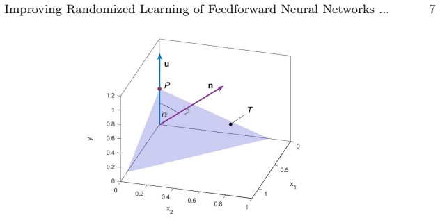
The load-bearing object is the slope angle $\alpha$: the angle between the tangent line (or hyperplane) to the sigmoid at its inflection point and the input axes. Because the sigmoid derivative at the inflection point is one quarter of the weight, the weight is recovered by $a = 4\tan\alpha$ in one dimension, and in $n$ dimensions the normal vector to the tangent hyperplane supplies both orientation and slope. The construction randomly draws the first $n$ normal components, fixes the remaining component from $\tan\alpha$, derives hidden weights, and then determines each bias so that the inflection point coincides with a randomly chosen training point or cluster prototype. This single mechanism keeps activation functions in their non-saturated regime and aligns their steep parts with the input distribution; $\alpha_{\min}$ is the new scalar that encodes target complexity.
What would settle it
Fit a one-dimensional target with rapid oscillation confined to a small subinterval and near-flat elsewhere, e.g. $g(x)=\sin(200x)$ on $[0,0.1]$ and $0$ on $(0.1,1]$, using the paper's Algorithm 1 with $\alpha_{\min}$ and $m$ tuned by cross-validation. If the error remains as low as on the paper's synthetic targets while the sigmoid inflection points are placed uniformly rather than concentrated in the oscillating region, the uniform-angle assumption holds; if not, that assumption is the part that fails.
Extended reading notes
Core claim
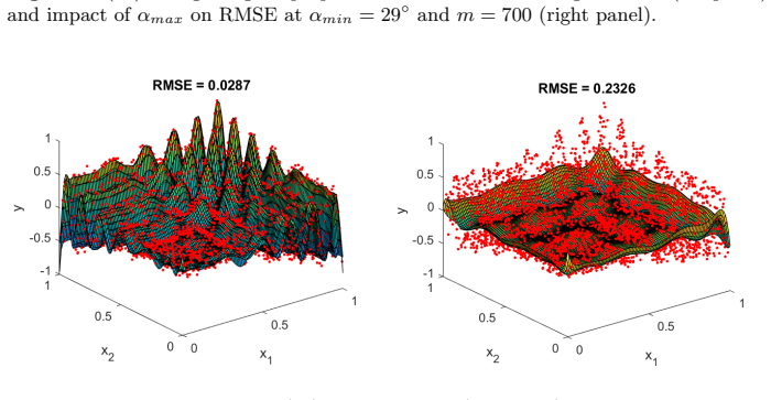
The central claim is that weights and biases of hidden nodes should not be sampled independently from the same fixed interval; they should be constructed so that the steep fragment of every sigmoid lands inside the input hypercube. For a one-input sigmoid the paper sets the weight by sampling the slope angle $\alpha$ at the inflection point and using $a = 4\tan\alpha$, then chooses the bias from $b_i = -a_i x^*_i$ so the inflection point sits at a randomly selected input point $x^*$. For multiple inputs, it builds a random tangent hyperplane to the sigmoid: the first $n$ components of the normal vector are drawn uniformly from $[-1,1]$, the last is fixed by $\cos\alpha = a'_0 / \sqrt{\sum a'_k{}^2}$, and the hidden weights follow $a_k = -4a'_k/a'_0$. This yields a set of constructional sigmoids that are steep, randomly oriented, and spread across the data. The paper reports test RMSE of $9.35\times 10^{-7}$ versus above $0.1$ on target (21), and $0.0287$ versus $0.2326$ on target (22); on the 21-dimensional Compactiv dataset the advantage shrinks to $0.0335$ versus $0.0358$, which the paper attributes to the absence of strong fluctuations.
Load-bearing premise
The method's edge depends on one global steepness interval, sampled uniformly, being able to supply every steepness the target function actually needs; if a target mixes very different local frequencies, the single limit angle $\alpha_{\min}$ can misplace or mis-size the steep sigmoids.
Editorial extensions
If this is right
- Hidden-node weights and biases should be treated as coupled quantities derived from the activation function's geometry, not as independent draws from one interval.
- A single cross-validated limit angle $\alpha_{\min}$ can replace a search over symmetric weight ranges, with $\alpha_{\max} = 90^\circ$ as a default.
- On strongly fluctuating target functions the method reaches test RMSE below $10^{-6}$ in the one-dimensional case and below $0.03$ in the two-dimensional case, while the fixed $[-1,1]$ baseline stays above $0.1$ and $0.23$.
- The advantage shrinks on smooth, high-dimensional data, so the method's benefit is concentrated precisely where randomized networks usually struggle.
Reading between the lines
- If the angle parameterization is the right prior, the fixed $[-1,1]$ weight interval may explain much of the excessive node counts and instability reported for randomized networks on nonlinear problems.
- The construction can be adapted to nonstationary targets by letting $\alpha_{\min}$ vary across the input space, using local estimates of fluctuation strength; the paper does not test this.
- The same geometry-based generation should carry over to other activation functions whose maximal derivative location is known, a direction the paper mentions only as future work.
- A plausible practical extension is to draw the rotation components from a narrower or wider interval to control the diversity of orientations, even though the paper recommends $[-1,1]$.
Signed reviews
Editorial analysis
A structured set of objections, weighed in public.
Referee Report
Summary. The paper proposes a method for generating the hidden-layer parameters of a single-hidden-layer feedforward network with random hidden nodes. Rather than drawing weights and biases from a fixed interval, it first samples a slope angle α for each sigmoid hidden node from an interval (α_min, α_max) chosen to match the target function's complexity, then computes the weight from a = 4 tan α in the one-dimensional case (or from a randomly rotated tangent hyperplane in the multidimensional case), and finally chooses the bias so that the sigmoid's inflection point lies at a randomly selected point inside the input hypercube. The method is illustrated on two synthetic regression functions and on the CompActiv data set; the reported test RMSEs are orders of magnitude smaller than those of the baseline that draws both weights and biases uniformly from [-1,1] for the synthetic functions, and slightly smaller on CompActiv.
Significance. The geometric rationale is clear and the algebraic derivation in Eqs. (3)-(8) and (11)-(19) is correct: the weight formula a = 4 tan α follows from the sigmoid derivative at the inflection point, and the bias formula b = -a^T x* correctly places the inflection point inside the input region. The procedure is interpretable and the hyperparameters are selected by standard cross-validation, with no circularity. If the empirical advantage were established against properly tuned baselines, the method would be a useful, practical alternative for randomized learning. However, the current evidence is not yet sufficient to support the central claim of substantial improvement, because the only comparator is an untuned fixed-interval baseline and no variability estimates are provided.
major comments (3)
- [Section 3] The central empirical claim is supported only by a comparison with the fixed-interval baseline a,b ∈ [-1,1]. As the paper itself notes in Section 1 (citing [5,6]), this interval is a known poor default; moreover, Eq. (5) shows that for the sigmoid in Eq. (2) weights in [-1,1] correspond to slope angles α ∈ [-14°,14°], i.e., deliberately flat basis functions, and biases in [-1,1] place many inflection points outside the input interval. The experiments therefore compare a cross-validated proposed method against an untuned special case rather than against standard randomized learning with a properly selected range. To support the abstract's claim, at least one baseline should tune the random-parameter range with the same cross-validation budget (e.g., the scaling factor s of [6] or the range optimization of [4]), and the comparison should include the author's earlier steepness-adjusted generation method [11].
- [Section 3, TFs (21) and (22)] No variability estimates are reported for the synthetic experiments. Because the hidden parameters are random, every learning session yields a different model, and the single RMSE values (9.35e-7 for TF (21) and 0.0287 for TF (22)) may not be representative. Repeat the experiments over many independent random parameter generations for both the proposed and baseline methods and report means and standard deviations; for CompActiv, the small difference (0.0335 vs 0.0358) should be accompanied by a statistical test.
- [Section 3, TF (21)] The selected optimum α_min = 85° lies at the edge of the searched grid shown in Fig. 3. Since the transformation a = 4 tan α diverges as α approaches 90°, a boundary optimum raises the concern that the headline result depends on an extreme hyperparameter value and that the grid search is not conclusive. Please extend the grid, constrain α_max, or otherwise demonstrate that the result is stable around the optimum.
minor comments (5)
- [Section 2.2, Eqs. (11)-(12), Algorithm 1] The definition of α as the angle between the normal vector n and the y-axis unit vector u requires a'_0 to be positive for α ∈ (0°,90°), yet Algorithm 1 chooses the sign of a'_0 randomly. Because the tangent hyperplane is invariant to a global sign change of n, the random sign is redundant and the notation becomes confusing; please either fix a'_0 > 0 or define α through |a'_0|.
- [Section 3, Eq. (21)] The text reports the optimum α_min = 85°, but the left panel of Fig. 3 appears to show a grid search only up to α_min = 80°; please clarify the grid range and the coordinate labels.
- [Section 3, TF (22)] There are apparent typos in the data-generation description: 'uniform noise distributed in [0.2, 0.2]' should presumably read [-0.2, 0.2], and 'normalized in the range [1, 1]' should presumably read [-1, 1].
- [Section 3, CompActiv] For the standard method on CompActiv, the number of hidden nodes is not stated; please report it and indicate whether the same m is used for both methods.
- [General] The paper does not provide code or a data repository, which would help reproducibility; please consider releasing the implementation and the exact hyperparameter grids.
Circularity Check
No circular derivation found: the parameter formulas follow from sigmoid calculus, and hyperparameters are selected by cross-validation rather than fitted to the reported test errors.
full rationale
The paper's generation rule is self-contained. Equation (5), a = 4 tan(alpha), is derived from the derivative of the logistic sigmoid at its inflection point (Equations 3-4). Equations (8) and (19), b_i = -sum a_{i,k} x*_k, follow from enforcing h(x*)=0.5, i.e. placing the inflection point at a chosen location inside the input hypercube. In the multidimensional case, Equation (12) is the geometry of the normal vector to the tangent hyperplane, and Equation (16) equates partial derivatives of the sigmoid with those of the tangent plane. None of these steps presupposes the target function or the reported error values. The hyperparameter alpha_min (and optionally alpha_max and m) is chosen by 10-fold cross-validation on the training set, and the reported errors are test-set errors (Section 3, Figures 3, 5, and 7). Thus the improvement claim is an empirical result against a fixed baseline, not a consequence of the construction. The self-citation [11] is background and is not used as the justification for the method's accuracy or as a uniqueness theorem. A separate concern is that the baseline [-1,1] is untuned, but that is a fairness/correctness issue, not circularity.
Assumptions & free parameters
free parameters (4)
- alpha_min =
85 deg for TF (21), 29 deg for TF (22), 45 deg for Compactiv
- alpha_max =
90 deg, except sensitivity analysis for TF (22)
- m (number of hidden nodes) =
320 for TF (21), 700 for TF (22), 600 for Compactiv
- d (rotation vector interval) =
1 (recommended)
assumptions (3)
- domain assumption Randomized single-hidden-layer FNNs with sigmoid hidden nodes and pseudo-inverse output weights are universal approximators
- domain assumption Sigmoid activation function is used and the derivation applies only to it
- ad hoc to paper Uniform sampling of slope angles is a suitable prior
Cite this review
Pith. "Pith review of Improving Randomized Learning of Feedforward Neural Networks by Appropriate Generation of Random Parameters." pith.science (2026). https://pith.science/paper/7UG7BNCL
@misc{pith2026190805542,
  author       = {Pith},
  title        = {Pith review of: Improving Randomized Learning of Feedforward Neural Networks by Appropriate Generation of Random Parameters},
  year         = {2026},
  howpublished = {\url{https://pith.science/paper/7UG7BNCL}},
  note         = {Machine review of arXiv:1908.05542}
}
read the original abstract
In this work, a method of random parameters generation for randomized learning of a single-hidden-layer feedforward neural network is proposed. The method firstly, randomly selects the slope angles of the hidden neurons activation functions from an interval adjusted to the target function, then randomly rotates the activation functions, and finally distributes them across the input space. For complex target functions the proposed method gives better results than the approach commonly used in practice, where the random parameters are selected from the fixed interval. This is because it introduces the steepest fragments of the activation functions into the input hypercube, avoiding their saturation fragments.
Figures


Figures from the paper (4 more)



Reference graph
Works this paper leans on
-
[5]
Information Sciences 382–383, 170–178 (2017)
Li, M., Wang, D.: Insights into randomized algorithms for neural networks: Practical issues and common pitfalls. Information Sciences 382–383, 170–178 (2017)
work page 2017
-
[6]
Information Sciences 367, 1094–1105 (2016)
Zhang, L., Suganthan, P.: A comprehensive evaluation of random vector functional link networks. Information Sciences 367, 1094–1105 (2016)
work page 2016
-
[11]
Information Sciences 481, 33–56 (2019)
Dudek, G.: Generating random weights and biases in feedforward neural networks with random hidden nodes. Information Sciences 481, 33–56 (2019)
work page 2019
-
[4]
Nurocomputing 6(2), 163–180 (1994)
Pao, Y.-H., Park, G.H., Sobajic, D.J.: Learning and generalization characteristics of the random vector functional-link net. Nurocomputing 6(2), 163–180 (1994)
work page 1994
-
[1]
Principe, J., Chen, B.: Universal approximation with convex optimization: Gimmick or reality? IEEE Comput Intell Mag 10, 68–77 (2015)
work page 2015
-
[2]
Igelnik, B., Pao, Y.-H.: Stochastic choice of basis functions in adaptive function ap- proximation and the functional-link net. IEEE Trans. Neural Networks 6(6), 1320– 1329 (1995)
work page 1995
-
[3]
Husmeier, D.: Random vector functional link (RVFL) networks. In: Neural Networks for Conditional Probability Estimation: Forecasting Beyond Point Predictions, chap- ter 6, 87–97, Springer-Verlag London (1999)
work page 1999
-
[7]
Wang D., Li, M.: Stochastic configuration networks: Fundamentals and algorithms. IEEE Trans. Cybernetics 47(10), 3466–3479 (2017)
work page 2017
Show all 12 references
-
[8]
Information Sciences 364, 146–155 (2016)
Gorban, A.N., Tyukin, I.Y., Prokhorov, D.V., Sofeikov, K.I.: Approximation with random bases: Pro- et contra. Information Sciences 364, 146–155 (2016)
2016
-
[9]
Information Sciences 364, 146–155 (2016)
Zhang, L., Suganthan, P.: A Survey of randomized algorithms for training neural networks. Information Sciences 364, 146–155 (2016)
2016
-
[10]
Neurocomputing 275, 278–287 (2018)
Weipeng, C., Wang, X., Ming, Z., Gao, J.: A review on neural networks with random weights. Neurocomputing 275, 278–287 (2018)
2018
-
[12]
WIREs Data Mining Knowl Discov 7 (2017)
Scardapane, S., Wang, D.: Randomness in neural networks: An overview. WIREs Data Mining Knowl Discov 7 (2017)
2017
Reviewed August 14, 2026 · model on record in the stance chip above.
Discussion (0). Continue with ORCID to comment.