REVIEW 3 major objections 4 minor 48 references
Fast Three-dimensional Opto-acoustic Simulation for Linear Array with Rectangular Elements
T0 review · 3 major / 4 minor · reviewed 2026-08-14 · deepseek-v4-flash
Pith's one-line read The 3D opto-acoustic response of a linear array with rectangular elements factors exactly into a cascade of two perpendicular 2D operators, an n-fold speedup.
desk verdict The separability proof holds up and the method is a real advance for homogeneous-fluence opto-acoustic simulation, but the fixed-fluence assumption and thin validation are the soft spots. read the letter →
The pith
A machine-rendered reading of the paper's core claim, the machinery that carries it, and where it could break.
The reading
What carries the argument
The load-bearing identity is the sifting factorization of the retarded Green's function, $$\delta(t-\|x\|)=\int_{-\infty}^{\infty}\delta(t-r)\delta(\tau-\rho)\,d\tau,\qquad r=\sqrt{$x_1^{2}$+\$tau^{2}$},\ \rho=\sqrt{$x_2^{2}$+$x_3^{2}$},$$ which decouples the 3D spherical wavefront into a circle in the $(x_2,x_3)$-plane followed by a circle in the $(x_1,\tau)$-plane. This factorization, together with changes of variables in the convolution integrals, is what carries the argument: it lets the system response operator be written as a composition, or cascade, of two operators, converting an $O(N)$ per-channel cost into $O(N^{2/3})$. The rectangular aperture enters through the multiplicatively separable form $f_1(u_1)f_2(u_2)\delta(u_3)$, so its two 1D factors can be paired with the two cascade stages.
What would settle it
Take a numerical phantom with a strongly absorbing inclusion placed between the light source and a second absorber, run the separable cascade and a dense non-separable reference simulation with the same fluence, and compare time traces; if the separable result differs from the reference by more than the known voxelization low-pass error, the factorization fails. A more direct check is to evaluate Proposition 3.1 on random volumes by computing $H^{A,b}$ directly as a 3D convolution and as the cascade $\tilde G\circ G^{A,b}$; any discrepancy beyond floating-point round-off would disprove the claimed identity.
Extended reading notes
Core claim
The central discovery is a separability theorem for the time-domain opto-acoustic operator. Writing the free-space pressure impulse response as $h(x,t)=\partial_t[\delta(t-\|x\|)/(4\pi t)]$, the paper factors the spherical shell $\delta(t-\|x\|)$ using a Dirac-delta identity into two nested circular integrations, one in a plane containing the array line and one perpendicular to it. This proves $H^{A,b} = \tilde G \circ G^{A,b}$: the first operator $G^{A,b}$ integrates the rotated and translated source over circles of radius $\tau$ in planes normal to the array, producing an intermediate function $\sigma$; the second operator $\tilde G$ integrates $\sigma$ over circles in the imaging plane and applies $\frac{1}{4\pi}\partial_t(1/t)$. For a multiplicatively separable rectangular aperture $f(u)=f_1(u_1)f_2(u_2)\delta(u_3)$, the two factors attach to the two cascade stages, so $H^{A,b}_f = \tilde G_{f_1}\circ G^{A,b}_{f_2}$. The obliquity factor is absorbed by weighting the source with $u_3$ before the cascade and by a $1/t$ post-factor, and a far-field variant rewrites the aperture convolution as six contour integrals, trading accuracy for speed.
Load-bearing premise
The load-bearing assumption is that the optical fluence $\Phi(u)$ stays fixed in the probe frame and is unaffected by local absorption variations, so heterogeneous tissue that significantly shadows deeper structures would break the model's description of the physical signal.
Editorial extensions
If this is right
- For a $512^3$ voxel volume, the reported GPU implementation runs a 256-channel, 1024-sample simulation on the order of real time, with the $n$-fold speedup growing as the volume side length grows.
- The same cascade, run in reverse, gives an adjoint operator usable for image reconstruction, since every forward step is linear and composable.
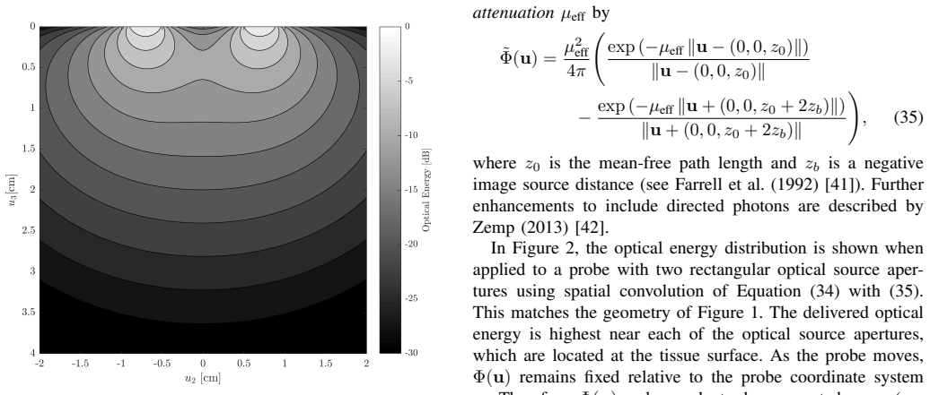
- Arbitrary probe positions and orientations are handled by the affine transform $T_{A,b}$: the volume is rotated and translated into the probe frame once, and the cached optical fluence $\Phi(u)$ does not need recomputation as the probe moves.
- The far-field contour approximation of Proposition 3.4 removes spatial convolutions with the aperture and can be faster at large grid sizes, at the cost of reduced near-field accuracy.
- The Dirac-delta proof of separability generalizes to any Green's-function kernel that is itself multiplicatively separable, extending the method beyond rectangular apertures.
Reading between the lines
- Editorial inference: Because the cascade is a composition of linear operators and each stage is shift-invariant along the array direction, the same factorization should carry over to linear inverse problems such as regularized maximum-likelihood reconstruction, where the system matrix could be applied implicitly as the product of the two sparse 2D kernels.
- Editorial inference: The fixed-fluence assumption is the main limitation; if absorption heterogeneity significantly perturbs the fluence, an iterative scheme could alternate the separable acoustic cascade with Monte Carlo or diffusion fluence updates, but the single-pass $n$-fold speedup would be lost. A testable middle ground is to precompute a small library of fluence maps for different bulk opt
- Editorial inference: The factoring identity suggests a direct numerical check of Green's-function separability in other wave-equation settings, such as weakly attenuating or dispersive media, by testing whether the factorized kernel reproduces the non-separable impulse response to machine precision on random volumes.
Signed reviews
Editorial analysis
A structured set of objections, weighed in public.
Referee Report
Summary. The paper develops a separable computational model for 3D opto-acoustic simulation with a linear array of rectangular transducer elements. Starting from the acoustic wave equation, it defines a generalized system response operator that includes the transducer aperture, an obliquity factor, a fixed optical energy distribution, and an affine transform to an arbitrarily rotated/translated probe frame. The central claim is that this non-separable 3D Green's function operator is equivalent to a cascade of two perpendicular 2D operators (Propositions 3.1-3.4), yielding an O(n) speedup for an n^3-voxel volume relative to a non-separable computation. The appendices contain proof sketches for each proposition, and a GPU implementation plus a point-source comparison against Field II are reported.
Significance. If the claims hold, the paper provides a valuable algebraic result: the 3D opto-acoustic forward operator, including rectangular-aperture impulse responses and obliquity weighting, can be evaluated as a cascade of two perpendicular 2D operations. The delta-function factorization in Eq. (36) and the grouping of aperture factors in Proposition 3.2 are nontrivial and internally consistent, and the complexity analysis (Table III) gives a clear O(N^{2/3}) scaling. The paper ships detailed proofs, a working GPU implementation, and reported runtimes for 128^3 to 768^3 volumes (Table II), which is a genuine strength. The main limitations are the fixed-fluence assumption, whose physical fidelity is not quantified, and the sparse accuracy validation against Field II.
major comments (3)
- [Section II.A, Eq. (9)] The stated change-of-coordinates identity is incorrect. With x = T_{A,b}(u) = Au+b, substituting y = T^{-1}_{A,b}(x') into the left-hand side gives ∫ h(y) ψ(A(u-y)) dy, while the right-hand side, using T^{-1}_{A,b}{ψ}(u) = ψ(Au+b) from Eq. (6b), gives ∫ h(y) ψ(A(u-y)+b) dy. The translation b does not appear on the left after the substitution. The correct relation is [T_{A,b}{h} ⊛ ψ](T_{A,b}(u)) = [h ⊛ (ψ∘A)](u), where (ψ∘A)(u) = ψ(Au). Because Eq. (9) is the stated motivation for the moving-frame operator definitions in Eqs. (19) and (30), this needs to be corrected and its consequences re-checked.
- [Section IV, Figures 7 and 8; Table II] The accuracy validation consists of a single point-source configuration at one depth, with no quantitative error metric reported; the difference from Field II is attributed only qualitatively to voxel-interpolation low-pass filtering. To support the abstract's claim of 'fast and accurate simulation,' the authors should report quantitative errors (e.g., normalized RMS or peak error) for multiple source depths, off-axis positions, and aperture widths, and include a rotated/translated probe test to validate the arbitrary-trajectory claim. In addition, Table II reports runtimes only for the separable implementation; a timing comparison against an actual non-separable implementation is needed to substantiate the claimed O(n) empirical speed-up.
- [Section II.C.3, Eqs. (31)-(33)] The generalized operator H^{A,b}_{f,Φ} is linear in η only under the stated assumption that Φ(u) is not affected by local changes in μ_a(x). The paper acknowledges this assumption but does not quantify its error in the intended breast-imaging regime, where blood-rich lesions with high absorption can perturb the fluence. If Φ depends on η, the mapping η→s is nonlinear and the operator formalism does not describe the physical signal. Please add a sensitivity analysis (e.g., comparing fixed-fluence simulations with Monte Carlo fluence recomputed for heterogeneous phantoms) or explicitly restrict the applicability claim in the abstract and conclusion to homogeneous or layered optical media.
minor comments (4)
- [Section IV, Figure 10 caption] The word 'diamter' should be 'diameter'.
- [Section III.D, Figure 4 caption] The caption does not define the solid and dotted lines in Figure 4b; please add a sentence stating which contour corresponds to the positive wavefront and which to the negative wavefront.
- [Table III and Table IV] The mixed-domain complexity entry uses parameters kd and ke, but Table IV defines ka, kb, kc, and kd but not ke; please define ke or remove it.
- [References] Reference [40] is cited as an unpublished manuscript to support the reconstructive utility of the separable operator; if it is not available, please label the relevant claim as future work or provide a linkable version.
Circularity Check
No significant circularity: the separable cascade is derived from the free-space Green's function and validated against an independent simulator; the fixed-fluence caveat is a modeling assumption, not a circular reduction.
full rationale
The central claim is the equivalence H^{A,b}_{f,Phi} = \tilde G_{f1} \circ G^{A,b}_{f2} (Propositions 3.1 and 3.2). The proof starts from the standard free-space pressure impulse response h(x,t) = (1/4\pi) \partial/\partial t [\delta(ct - ||x||)/t] and uses the delta-function factorization in Eq. (36), \delta(t - ||x||) = \int \delta(t-r)\delta(\tau-\rho)\,d\tau, followed by polar-coordinate changes of variables. The operators G and \tilde G are defined by these derived integrals, not by imposing the desired output, so the separability result is a genuine mathematical derivation rather than a definitional equivalence. Rectangular-aperture separability follows from f_a(x) = rect(x1/a1, x2/a2)\delta(x3) and convolution associativity, and the obliquity-factor case is derived from the identity \nabla g(x,t)\cdot\hat n = h(x,t)\alpha(x)/c0 (Proposition 3.3). No fitted parameter is renamed as a prediction: the optical energy distribution Phi(u) is an input computed from standard diffusion or Monte-Carlo optical models, and the transducer impulse response is not tuned to match the Field II output used for validation. The self-citations, e.g., references [7] and [40], are to the authors' reconstruction-related follow-ups and are not needed to establish the separability claim. The fixed-fluence assumption stated in Section II.C.3, that Phi(u) is not affected by local changes in optical absorption mu_a(x), is explicitly acknowledged and limits physical fidelity in heterogeneous tissue, but it is a modeling assumption rather than a circular step. The numerical comparison to the independent Field II simulator provides external validation of the derived impulse responses. No step in the chain reduces by construction to its own inputs.
Assumptions & free parameters
assumptions (6)
- domain assumption Acoustic medium is homogeneous with constant speed of sound and density.
- domain assumption Optical energy distribution Phi(u) is independent of local absorption and fixed relative to the probe frame.
- domain assumption Instantaneous optical pulse q(t) = delta(t).
- standard math Free-space Green's function solution to the 3D scalar wave equation.
- domain assumption Rectangular transducer aperture is multiplicatively separable: f(u) = f1(u1) f2(u2) delta(u3).
- standard math Sifting, scaling and composition properties of the Dirac delta function.
Cite this review
Pith. "Pith review of Fast Three-dimensional Opto-acoustic Simulation for Linear Array with Rectangular Elements." pith.science (2026). https://pith.science/paper/WXQBVNK6
@misc{pith2026190805581,
  author       = {Pith},
  title        = {Pith review of: Fast Three-dimensional Opto-acoustic Simulation for Linear Array with Rectangular Elements},
  year         = {2026},
  howpublished = {\url{https://pith.science/paper/WXQBVNK6}},
  note         = {Machine review of arXiv:1908.05581}
}
abstract
Simulation involves predicting responses of a physical system. In this article, we simulate opto-acoustic signals generated in a three-dimensional volume due to absorption of an optical pulse. A separable computational model is developed that permits an order-of-magnitude improvement in computational efficiency over a non-separable model. The simulated signals represent acoustic waves, measured by a probe with a linear transducer array, in a rotated and translated coordinate frame. Light is delivered by an optical source that moves with the probe's frame. A spatio-temporal impulse response for rectangular element transducer geometry is derived using a Green's function solution to the acoustic wave equation. The approach permits fast and accurate simulation for a probe with arbitrary trajectory. For a 3D volume of $n^3$ voxels, computation is accelerated by a factor of $n$. This may potentially have application for opto-acoustic imaging, where clinicians visualize structural and functional features of biological tissue for assessment of cancer and other diseases.
Figures


Figures from the paper (5 more)


Reference graph
Works this paper leans on
-
[1]
AA Oraevsky, B Clingman, J Zalev, AT Stavros, WT Yang, and JR Parikh. “Clinical optoacoustic imaging combined with ultrasound for coregistered functional and anatomical mapping of breast tumors”. In: Photoa- coustics 12 (2018), pp. 30–45
work page 2018
-
[2]
Opto-acoustic image fusion technology for diagnostic breast imaging in a feasibility study
Jason Zalev, Bryan Clingman, Don Herzog, Tom Miller, Michael Ulissey, A Thomas Stavros, Alexander Oraevsky, Philip Lavin, Kenneth Kist, N Carol Dorn- bluth, and Pamela Otto. “Opto-acoustic image fusion technology for diagnostic breast imaging in a feasibility study”. In: SPIE Medical Imaging. International Society for Optics and Photonics. 2015, pp. 941909–941909
work page 2015
-
[3]
E I Neuschler, R Butler, C A Young, L D Barke, M L Bertrand, M B ¨ohm-V´elez, S Destounis, P Donlan, S R Grobmyer, J Katzen, K A Kist, P T Lavin, E V Makariou, T M Parris, K J Schilling, F L Tucker, and B E Dogan. “A Pivotal Study of Optoacoustic Imaging to Diagnose Benign and Malignant Breast Masses: A New Evaluation Tool for Radiologists.” In: Radiology...
work page 2018
-
[4]
Downgrading of Breast Masses Suspicious for Cancer by Using Optoacoustic Breast Imaging
Gisela LG Menezes, Ruud M Pijnappel, Carla Meeuwis, Robertus Bisschops, Jeroen Veltman, Philip T Lavin, Marc J van de Vijver, and Ritse M Mann. “Downgrading of Breast Masses Suspicious for Cancer by Using Optoacoustic Breast Imaging”. In: Radiology (2018), p. 170500
work page 2018
-
[5]
Optoacoustic tomography: from fundamentals to diagnostic imaging of breast can- cer
Alexander A Oraevsky. “Optoacoustic tomography: from fundamentals to diagnostic imaging of breast can- cer”. In: Biomedical Photonics Handbook . CRC press, 2014, pp. 738–781
work page 2014
-
[6]
Photoacoustic imag- ing in biomedicine
Minghua Xu and Lihong V Wang. “Photoacoustic imag- ing in biomedicine”. In: Review of scientific instruments 77.4 (2006), p. 041101
work page 2006
-
[7]
Image Reconstruction Combined with Interference Removal using a Mixed- Domain Proximal Operator
Jason Zalev and Michael Kolios. “Image Reconstruction Combined with Interference Removal using a Mixed- Domain Proximal Operator”. In: IEEE Signal Process- ing Letters (2018)
work page 2018
-
[8]
Philip McCord Morse and K Uno Ingard. Theoretical acoustics. Princeton university press, 1968
work page 1968
Show all 48 references
-
[9]
Application of time-space impulse responses to calculations of acoustic fields in imaging systems
Henryk Lasota and Roman Salamon. “Application of time-space impulse responses to calculations of acoustic fields in imaging systems”. In: Acoustical Imaging . Springer, 1982, pp. 493–512
1982
-
[10]
A the- ory for the radiation pattern of a narrow-strip acoustic transducer
AR Selfridge, GS Kino, and BT Khuri-Yakub. “A the- ory for the radiation pattern of a narrow-strip acoustic transducer”. In: Applied Physics Letters 37.1 (1980), pp. 35–36
1980
-
[11]
Field: A program for simulating ultrasound systems
Jørgen Arendt Jensen. “Field: A program for simulating ultrasound systems”. In: 10th Nordicbaltic Conference on Biomedical Imaging, Vol. 4, Supplement 1, Part 1: 351–353. Citeseer. 1996
1996
-
[12]
Cal- culation of pressure fields from arbitrarily shaped, apodized, and excited ultrasound transducers
Jørgen Arendt Jensen and Niels Bruun Svendsen. “Cal- culation of pressure fields from arbitrarily shaped, apodized, and excited ultrasound transducers”. In: IEEE transactions on ultrasonics, ferroelectrics, and fre- quency control 39.2 (1992), pp. 262–267
1992
-
[13]
Transient radiation from pistons in an infinite planar baffle
Peter R Stepanishen. “Transient radiation from pistons in an infinite planar baffle”. In: The Journal of the Acoustical Society of America 49.5B (1971), pp. 1629– 1638
1971
-
[14]
Acoustic diffraction analysis by the impulse response method: A line impulse response approach
H Lasota, R Salamon, and B Delannoy. “Acoustic diffraction analysis by the impulse response method: A line impulse response approach”. In: The Journal of the Acoustical Society of America 76.1 (1984), pp. 280– 290
1984
-
[15]
A new approach to the derivation of the impulse response of a rectangular piston
G Scarano, N Denisenko, M Matteucci, and M Pap- palardo. “A new approach to the derivation of the impulse response of a rectangular piston”. In: The Jour- nal of the Acoustical Society of America 78.3 (1985), pp. 1109–1113
1985
-
[16]
Diffraction impulse response of rectangular transducers
Jose Luis San Emeterio and Luis G Ullate. “Diffraction impulse response of rectangular transducers”. In: The Journal of the Acoustical Society of America 92.2 (1992), pp. 651–662
1992
-
[17]
Two-pass 3D migration and linearized inversion in the (x, t)-domain
H Jakubowicz and D Miller. “Two-pass 3D migration and linearized inversion in the (x, t)-domain”. In: Geo- physical prospecting 37.2 (1989), pp. 143–148
1989
-
[18]
Basic earth imaging
Jon F Claerbout and I Green. Basic earth imaging. 2008
2008
-
[19]
Ul- trasound transducers for pulse-echo medical imaging
John W Hunt, Marcel Arditi, and F Stuart Foster. “Ul- trasound transducers for pulse-echo medical imaging”. In: IEEE Transactions on Biomedical Engineering 8 (1983), pp. 453–481
1983
-
[20]
Foundations of biomedical ultra- sound
Richard SC Cobbold. Foundations of biomedical ultra- sound. Oxford University Press, 2006. 22 J. Zalev and M. C. Kolios
2006
-
[21]
Comments on “Farfield of Pulsed Rectangular Acoustic Radiator
PR Stepanishen. “Comments on “Farfield of Pulsed Rectangular Acoustic Radiator”[A. Freedman, J. Acoust. Soc. Amer. 49, 738–748 (1971)]”. In: The Journal of the Acoustical Society of America 52.1B (1972), pp. 434–436
1971
-
[22]
Farfield of pulsed rectangular acous- tic radiator
Albert Freedman. “Farfield of pulsed rectangular acous- tic radiator”. In: The Journal of the Acoustical Society of America 49.3B (1971), pp. 738–748
1971
-
[23]
Rapid calculations of time- harmonic nearfield pressures produced by rectangular pistons
Robert J McGough. “Rapid calculations of time- harmonic nearfield pressures produced by rectangular pistons”. In: The Journal of the Acoustical Society of America 115.5 (2004), pp. 1934–1941
2004
-
[24]
A 2D fast near-field method for calculating near-field pressures generated by apodized rectangular pistons
Duo Chen and Robert J McGough. “A 2D fast near-field method for calculating near-field pressures generated by apodized rectangular pistons”. In: The Journal of the Acoustical Society of America 124.3 (2008), pp. 1526– 1537
2008
-
[25]
An efficient grid sectoring method for calcula- tions of the near-field pressure generated by a circular piston
Robert J McGough, Thaddeus V Samulski, and James F Kelly. “An efficient grid sectoring method for calcula- tions of the near-field pressure generated by a circular piston”. In: The Journal of the Acoustical Society of America 115.5 (2004), pp. 1942–1954
2004
-
[26]
A simple exact method of 3-D migration theory
H Jakubowicz and S Levin. “A simple exact method of 3-D migration theory”. In: Geophysical Prospecting 31.1 (1983), pp. 34–56
1983
-
[27]
Com- ments on
JT Fokkema, GJM L ¨ortzer, and AM Ziolkowski. “Com- ments on ”A simple exact method of (3-D) migration theory” by H. Jakubowicz and S. Levin–a note in favour of ”The myth of nonseparability of the (3-D) migration operator””. In: Geophysical prospecting 34.6 (1986), pp. 927–936
1986
-
[28]
The k-space formulation of the scattering problem in the time domain
Norbert N Bojarski. “The k-space formulation of the scattering problem in the time domain”. In: The Jour- nal of the Acoustical Society of America 72.2 (1982), pp. 570–584
1982
-
[29]
k-space propagation models for acoustically heterogeneous media: Application to biomedical pho- toacoustics
Benjamin T Cox, S Kara, Simon R Arridge, and Paul C Beard. “k-space propagation models for acoustically heterogeneous media: Application to biomedical pho- toacoustics”. In: The Journal of the Acoustical Society of America 121.6 (2007), pp. 3453–3464
2007
-
[30]
Fast calculation of pulsed photoacoustic fields in fluids using k-space methods
BT Cox and PC Beard. “Fast calculation of pulsed photoacoustic fields in fluids using k-space methods”. In: The Journal of the Acoustical Society of America 117.6 (2005), pp. 3616–3627
2005
-
[31]
k-Wave: MATLAB toolbox for the simulation and reconstruction of photoacoustic wave fields
Bradley E Treeby and Benjamin T Cox. “k-Wave: MATLAB toolbox for the simulation and reconstruction of photoacoustic wave fields”. In: Journal of biomedical optics 15.2 (2010), p. 021314
2010
-
[32]
Application of inverse source concepts to photoacoustic tomography
Mark A Anastasio, Jin Zhang, Dimple Modgil, and Patrick J La Rivi `ere. “Application of inverse source concepts to photoacoustic tomography”. In: Inverse Problems 23.6 (2007), S21
2007
-
[33]
Analytic expla- nation of spatial resolution related to bandwidth and detector aperture size in thermoacoustic or photoacous- tic reconstruction
Minghua Xu and Lihong V Wang. “Analytic expla- nation of spatial resolution related to bandwidth and detector aperture size in thermoacoustic or photoacous- tic reconstruction”. In: Physical Review E 67.5 (2003), p. 056605
2003
-
[34]
An imaging model incorporating ultrasonic transducer properties for three-dimensional optoacoustic tomogra- phy
Kun Wang, Sergey A Ermilov, Richard Su, Hans-Peter Brecht, Alexander A Oraevsky, and Mark A Anastasio. “An imaging model incorporating ultrasonic transducer properties for three-dimensional optoacoustic tomogra- phy”. In: IEEE transactions on medical imaging 30.2 (2011), pp. 203–214
2011
-
[35]
Investigation of the far-field approximation for model- ing a transducer’s spatial impulse response in photoa- coustic computed tomography
Kenji Mitsuhashi, Kun Wang, and Mark A Anastasio. “Investigation of the far-field approximation for model- ing a transducer’s spatial impulse response in photoa- coustic computed tomography”. In: Photoacoustics 2.1 (2014), pp. 21–32
2014
-
[36]
Accelerating image reconstruction in three- dimensional optoacoustic tomography on graphics pro- cessing units
Kun Wang, Chao Huang, Yu-Jiun Kao, Cheng-Ying Chou, Alexander A Oraevsky, and Mark A Anas- tasio. “Accelerating image reconstruction in three- dimensional optoacoustic tomography on graphics pro- cessing units”. In: Medical physics 40.2 (2013)
2013
-
[37]
L1-L2 opti- mization in signal and image processing
Michael Zibulevsky and Michael Elad. “L1-L2 opti- mization in signal and image processing”. In: IEEE Signal Processing Magazine 27.3 (2010), pp. 76–88
2010
-
[38]
Biomedical Image Reconstruction: From the Foundations to Deep Neural Networks
Michael T McCann, Michael Unser, et al. “Biomedical Image Reconstruction: From the Foundations to Deep Neural Networks”. In: Foundations and Trends® in Signal Processing 13.3 (2019), pp. 283–359
2019
-
[39]
The application of compressed sensing for photo-acoustic tomography
Jean Provost and Fr ´ed´eric Lesage. “The application of compressed sensing for photo-acoustic tomography”. In: IEEE transactions on medical imaging 28.4 (2009), pp. 585–594
2009
-
[40]
Opto-acoustic Image Recon- struction and Motion Tracking using Convex Optimiza- tion
J. Zalev and M.C. Kolios. “Opto-acoustic Image Recon- struction and Motion Tracking using Convex Optimiza- tion”. Unpublished manuscript, Department of Physics, Ryerson University, Toronto, Canada. 2020
2020
-
[41]
A diffusion theory model of spatially resolved, steady-state diffuse reflectance for the noninvasive de- termination of tissue optical properties in vivo
Thomas J Farrell, Michael S Patterson, and Brian Wil- son. “A diffusion theory model of spatially resolved, steady-state diffuse reflectance for the noninvasive de- termination of tissue optical properties in vivo”. In: Medical physics 19.4 (1992), pp. 879–888
1992
-
[42]
Phase-function corrected diffusion model for diffuse reflectance of a pencil beam obliquely incident on a semi-infinite turbid medium
Roger J Zemp. “Phase-function corrected diffusion model for diffuse reflectance of a pencil beam obliquely incident on a semi-infinite turbid medium”. In: Journal of biomedical optics 18.6 (2013), p. 067005
2013
-
[43]
Light transport in three-dimensional semi-infinite scattering media
Andr ´e Liemert and Alwin Kienle. “Light transport in three-dimensional semi-infinite scattering media”. In: JOSA A 29.7 (2012), pp. 1475–1481
2012
-
[44]
Analytical approach for solving the radiative transfer equation in two- dimensional layered media
Andr ´e Liemert and Alwin Kienle. “Analytical approach for solving the radiative transfer equation in two- dimensional layered media”. In: Journal of Quantita- tive Spectroscopy and Radiative Transfer 113.7 (2012), pp. 559–564
2012
-
[45]
Comparison of finite-difference trans- port and diffusion calculations for photon migration in homogeneous and heterogeneous tissues
Andreas H Hielscher, Raymond E Alcouffe, and Ran- dall L Barbour. “Comparison of finite-difference trans- port and diffusion calculations for photon migration in homogeneous and heterogeneous tissues”. In: Physics in Medicine & Biology 43.5 (1998), p. 1285
1998
-
[46]
MCML—Monte Carlo modeling of light transport in multi-layered tissues
Lihong Wang, Steven L Jacques, and Liqiong Zheng. “MCML—Monte Carlo modeling of light transport in multi-layered tissues”. In: Computer methods and programs in biomedicine 47.2 (1995), pp. 131–146. 23 J. Zalev and M. C. Kolios
1995
-
[47]
A Monte Carlo model for the absorption and flux distributions of light in tissue
BC Wilson and G Adam. “A Monte Carlo model for the absorption and flux distributions of light in tissue”. In: Medical physics 10.6 (1983), pp. 824–830
1983
-
[48]
Shanghai Lectures on Multivariable Analysis
William G Faris. Shanghai Lectures on Multivariable Analysis . Online Book. http://math.arizona.edu/ faris/books.html, 2016. 24 J. Zalev and M. C. Kolios
2016
Reviewed August 14, 2026 · model on record in the stance chip above.
Discussion (0). Continue with ORCID to comment.