Learning Signal Subgraphs from Longitudinal Brain Networks with Symmetric Bilinear Logistic Regression

Lu Wang; Zhengwu Zhang

REVIEW 4 major objections 5 minor 26 references

Learning Signal Subgraphs from Longitudinal Brain Networks with Symmetric Bilinear Logistic Regression

T0 review · 4 major / 5 minor · reviewed 2026-08-14 · deepseek-v4-flash

Challenge this review Re-run · record.json Download PDF Read on arXiv ↗ Review JSON

Pith's one-line read A symmetric bilinear logistic regression learns small clique subgraphs from longitudinal brain networks and estimates how each subgraph's predictive weight changes with age; on ADNI connectomes it identifies a frontal- and temporal-pole…

desk verdict A solid methodological extension with a credible derivational core, but the headline ADNI predictive claim is under-quantified and may be leaky; referee it, but expect revisions. read the letter →

arxiv 1908.05627 v1 pith:3YFTEFJ2 submitted 2019-08-15 stat.AP q-bio.NC

Lu Wang , Zhengwu Zhang This is my paper · ORCID

classification stat.APq-bio.NC

keywords signalsubgraphlearninglongitudinalbrainnetworkssymmetricbilinearlogisticregressioncliquesubgraphsageeffectstructuralconnectomicselastic-netpenaltysupernormalaging

verification ladder T0 review T1 audit T2 compute T3 formal

The pith

A machine-rendered reading of the paper's core claim, the machinery that carries it, and where it could break.

The reading

This paper proposes a way to predict a binary trait from a set of longitudinal brain networks, treating each network as a matrix predictor rather than a bag of edges. The model, symmetric bilinear logistic regression (SBLR), represents each outcome-relevant subgraph as a rank-one symmetric matrix $\beta_h \beta_h^\top$, so the selected connections form a clique—a small set of mutually connected brain regions that can be read as a neurological circuit. A scalar function $\lambda_h(g) = \gamma_h g^2 + \rho_h g + \alpha_h$ multiplies each clique and lets its predictive weight change with age while the subgraph itself stays fixed. On ADNI structural connectomes, SBLR identifies a frontal-pole-centered clique whose connection strength is positively associated with "supernormal" cognitive aging, and it reports lower cross-validated deviance than an unstructured logistic-regression baseline. The payoff, if correct, is that a high-dimensional edge-selection problem collapses to a few interpretable circuits with estimable age trajectories.

What carries the argument

The central object is the rank-one symmetric coefficient matrix $\beta_h \beta_h^\top$ inside a logistic link. Its nonzero off-diagonal entries mark the edges of a clique subgraph, so each component selects a set of mutually connected nodes that can be interpreted as a circuit; the age effect is carried by a scalar polynomial $\lambda_h(g) = \gamma_h g^2 + \rho_h g + \alpha_h$ multiplying the whole clique. With $\lambda_h$ quadratic, the longitudinal predictor collapses into three per-subject matrix averages: $\frac{1}{T_i} \sum_s W_i^{(s)}$, $\frac{1}{T_i} \sum_s g_{is} W_i^{(s)}$, and $\frac{1}{T_i} \sum_s g_{is}^2 W_i^{(s)}$, which is what lets the method handle subjects with different numbers of visits. Estimation uses coordinate descent with an entrywise elastic-net penalty whose per-entry weight grows with the current $\ell^1$ mass of the rest of the component, pushing unnecessary components to zero and keeping the selected subgraphs small; the loss is not jointly concave in $\beta_h$, but each coordinate update is convex.

What would settle it

Refit or evaluate the model on age-banded subsets of the ADNI data, for example subjects seen near ages 60-70 versus 80-95, allowing the subgraph membership $\beta_h$ to be re-estimated within each band. If the same frontal- and temporal-pole clique does not predict supernormal status in every band, or if a different clique is selected, the fixed-subgraph assumption is violated and the reported age effect is an artifact of averaging.

Watch

Extended reading notes

Core claim

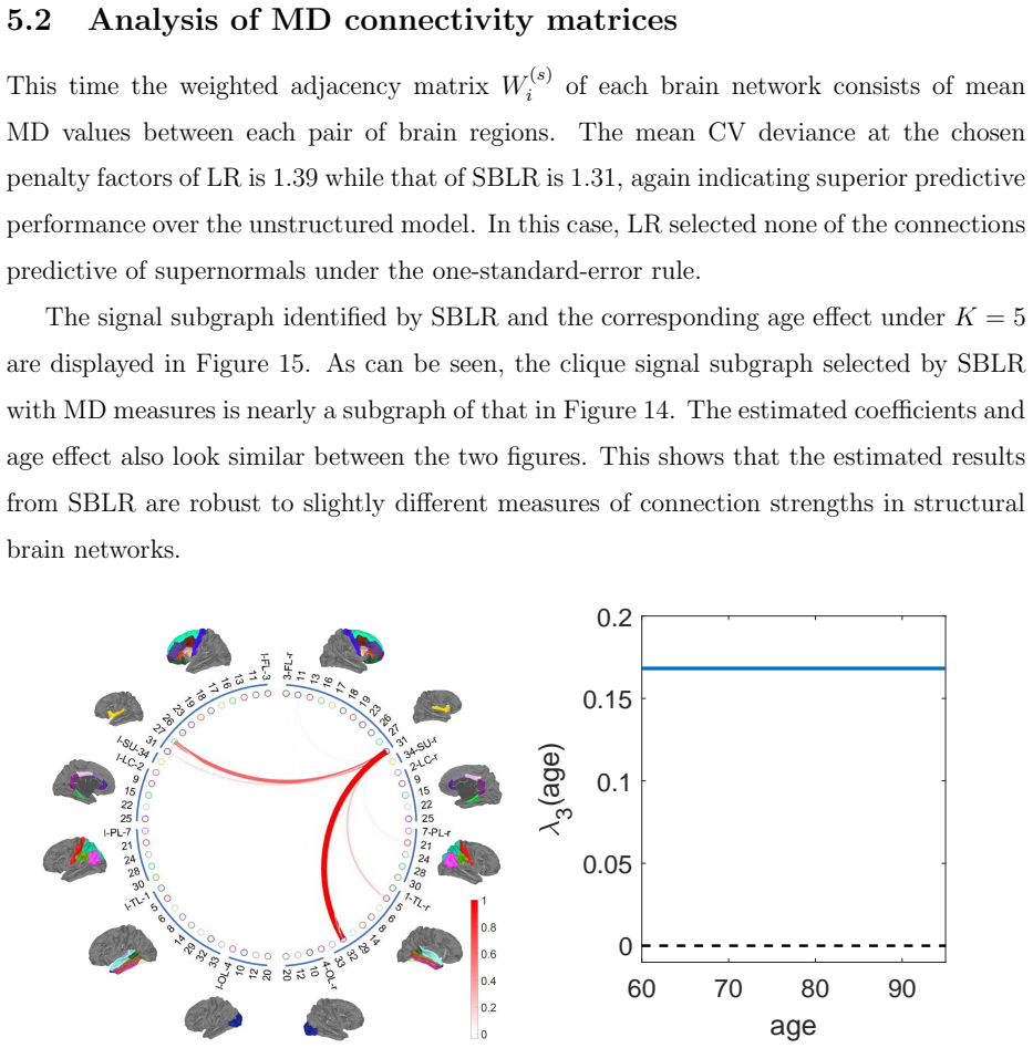
On the paper's own terms, the central discovery is that a logistic model with components $\mathrm{logit}(p_i) = \alpha_0 + \sum_{h=1}^K \frac{1}{T_i} \sum_{s=1}^{T_i} \lambda_h(g_{is}) \beta_h^\top W_i^{(s)} \beta_h$ can simultaneously select sparse clique subgraphs and estimate their age effects from longitudinal networks with irregular visit schedules. Because each component's coefficient matrix is $\lambda_h(g) \beta_h \beta_h^\top$, nonzero off-diagonal entries sit exactly on a clique, and the shared quadratic $\lambda_h(g)$ captures how that circuit's contribution to the outcome drifts with age. Simulations show the method recovers true signal edges with the lowest false-positive rate among SBLR, unstructured elastic-net logistic regression, and a tensor-regression baseline, while matching or beating them in out-of-sample deviance. In the ADNI application, SBLR selects one clique around the frontal pole, with superior frontal and temporal pole nodes, whose connection strengths are positively and constantly associated with supernormal status across ages, with mean cross-validated deviance 1.29 (FA) and 1.31 (MD) versus 1.38 and 1.39 for the unstructured logistic regression.

Load-bearing premise

The load-bearing premise is that the brain regions and their connections in each signal subgraph stay the same for everyone across all ages; the model only lets the statistical weight of each fixed circuit change with age.

Editorial extensions

If this is right

A handful of clique subgraphs, each tied to named anatomy, can replace long edge lists in longitudinal brain-outcome studies.
Subjects with different numbers of visits can be pooled without imputation, because the model uses per-subject averages of the network, the age-weighted network, and the age-squared-weighted network.
The estimated $\hat{\lambda}_h(g)$ gives a population-level trajectory of how a circuit's predictive weight changes with age; a constant trajectory means no age window is especially decisive.
The same clique emerges from fractional anisotropy and mean diffusivity connectomes, suggesting the finding is not an artifact of one diffusion measure.
SBLR is conservative relative to unstructured elastic-net regression, favoring fewer false-positive edges at comparable predictive deviance.

Reading between the lines

Editorial extensions of the paper, not claims the author makes directly.

A stronger test of the paper's stability assumption would let $\beta_h$ vary by age window, for example 60-74 versus 75-95; the current model only varies $\lambda_h$, so the inference that the same circuit operates throughout aging is not directly tested.
The identified frontal-pole-centered circuit generates a concrete prediction for independent cohorts: white-matter integrity among frontal pole, superior frontal, and temporal pole regions should track memory performance in older adults classified as superagers.
The per-subject averaging trick could be reused for functional connectomes, such as fMRI, after aligning visits to age bins, making the same logistic-bilinear construction applicable beyond diffusion MRI.

Share X Bluesky LinkedIn Reddit HN

Signed reviews

No signed human review yet.

Editorial analysis

A structured set of objections, weighed in public.

Desk editor's note, referee report, and a circularity audit.

Desk Editor's Note

read the letter

The new thing here is a logistic regression extension of the authors' earlier symmetric bilinear model, now handling longitudinal network predictors and age-varying coefficients. The coordinate descent derivations are explicit, the per-iteration complexity analysis is honest, and the sparsity/interpretability benefit over unstructured elastic-net regression comes through in the simulations. Code is on GitHub, which helps. The soft spots are real but mostly addressable. The biggest one is the application section. The abstract says SBLR beats competitors on ADNI, but the evidence is only two point estimates of mean CV deviance (1.29 vs 1.38 for FA; 1.31 vs 1.39 for MD) with n=85. No standard errors, no repeated splits. A difference of 0.08–0.10 is well within plausible sampling noise at that sample size. Worse, Section 3 describes normalizing the edge weights and age terms on the observations before model fitting, and Section 3.5 then does 5-fold CV. If that normalization was computed on pooled data, the fold structure is breached and the CV deviance is optimistically biased. The paper never states that normalization is fold-aware. That is the load-bearing weakness in the headline claim. Two smaller things. First, the convergence guarantee is asserted rather than proven: the algorithm uses a quadratic approximation in coordinate descent, and while the loss is lower bounded, that alone does not guarantee each update decreases it. A line search or a proper majorization argument would settle it. Second, Table 1 contains an unexplained value: under n=1000, SBLR has mean CV deviance 0.1767 while LR and NSTR are around 1.18. That looks like a typo, and it makes the whole table harder to trust. The temporal stability assumption on the subgraphs is explicit and reasonable as a first model, though it should be flagged more prominently as a limitation in the discussion. The methodological core is sound and the simulation protocol is sensible. The paper is an incremental but useful tool for connectomics researchers who want sparse, interpretable subgraph regression for binary outcomes. It deserves a serious referee. My recommendation: send it to peer review, but the application section needs fold-aware preprocessing, uncertainty quantification on the CV deviance, and a corrected Table 1 before publication.

Referee Report

4 major / 5 minor

Summary. The paper proposes symmetric bilinear logistic regression (SBLR) for binary outcomes from longitudinal brain networks. The model assumes that a small number of outcome-relevant signal subgraphs are captured by component vectors β_h, and that the predictive effect of each subgraph evolves with age through a shared quadratic function λ_h(g) = γ_h g^2 + ρ_h g + α_h. An elastic-net penalty on the lower-triangular entries of λ_h(g) β_h β_h^T encourages sparse clique subgraphs. Estimation is performed by a coordinate descent algorithm with quadratic approximations, and model selection uses 5-fold cross-validation with a one-standard-error rule. Simulations compare SBLR with unstructured logistic regression and a naively symmetrized tensor regression. An application to ADNI data with FA and MD connectivity matrices identifies a frontal/temporal-pole subgraph and reports lower mean CV deviance for SBLR than for logistic regression.

Significance. If the claims hold, the paper offers a useful structured alternative to edge-wise logistic regression for longitudinal network predictors, with interpretable clique subgraphs and population-level age effects. The coordinate-wise update derivations are explicit, the simulation protocol is sensible, and the authors provide publicly available code, which are strengths. The method is an incremental but nontrivial extension of Wang et al. (2019) to binary longitudinal outcomes with age-varying effects. However, the empirical support for the headline claim of "better predictive performance than competitors" is currently thin: the reported CV deviance differences in the application are unquantified, the preprocessing may leak information into cross-validation, and the convergence guarantee is asserted rather than proved. These issues are fixable but need to be addressed before the paper can be accepted.

major comments (4)

[§5.1 and §5.2] The abstract and Section 5 claim "better predictive performance than competitors" based on point estimates of mean CV deviance: SBLR 1.29 versus LR 1.38 for FA, and SBLR 1.31 versus LR 1.39 for MD. With n = 85 and balanced classes, these differences are within plausible sampling noise, and no fold-level variability, repeated-split estimates, or paired comparison is provided. Report standard errors or confidence intervals for the CV deviance (or a paired test across folds) and temper the predictive-performance claim accordingly.
[§3 and §3.5] The preprocessing described at the start of Section 3 standardizes the raw network entries and age terms over "the observations" before model fitting, and Section 3.5 then performs 5-fold CV for tuning. If this standardization is computed on the pooled data before the folds are formed, held-out subjects' edge means and variances leak into the training predictors, biasing the CV deviance optimistically. Clarify whether normalization is fold-aware; if it is not, repeat the evaluation with within-training-fold standardization and report whether the conclusions change.
[§3.4] The convergence guarantee is asserted rather than proved: "Since the loss function (5) is lower bounded by 0 and each update always decreases the function value, the coordinate descent algorithm derived above is guaranteed to converge." Each update in equations (17)–(26) minimizes a second-order Taylor approximation of the loss, not the true loss, so monotone decrease of the true objective is not automatic. Provide a descent lemma or modify the algorithm (for example, with an exact coordinate minimization or a line search) to make the convergence claim rigorous.
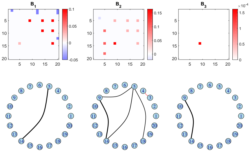
[§4.2, Table 1] The simulation evidence for signal-subgraph recovery is weaker than the narrative suggests: at n = 100 the mean TPR for SBLR is 0.219 (K = 5) with SD 0.271, and the displayed run recovers only part of one of the two true subgraphs. The conclusion that SBLR "learns" signal subgraphs should be framed as partial recovery with strong false-positive control, or additional simulation configurations with stronger signal-to-noise ratio should be considered to substantiate the recovery claim.

minor comments (5)

[§3.4] The word "summerized" in Algorithm 1's description should be "summarized".
[§4.2, Figure 8] The middle panel says "red edges ... (not displayed)"; this parenthetical contradicts the legend and should be removed or the red edges should be shown.
[§3.5] The definition of δ_min as "a sufficiently small value that produces dense results" is vague; give an operational definition or a default formula for choosing the grid endpoints.
[§2] The identifiability of the elastic-net penalty is motivated by a reference to Wang et al. (2019); a brief self-contained statement of the identifiability argument for the logistic and longitudinal setting would help readers.
[§5] In the application, SBLR is compared only with LR, not with NSTR or other structured competitors; the abstract's plural "competitors" overstates the scope of the empirical comparison.

Circularity Check

0 steps flagged · score 0.0 of 10

No significant circularity: the SBLR derivation is self-contained, and the one self-citation is technical support, not a reduced prediction.

full rationale

The core model is introduced directly: logit(pi) is stated as a logistic generalization of the symmetric bilinear form with longitudinal averaging (Eq. 1), the quadratic age effect is plugged in explicitly (Eq. 3), and the elastic-net objective is written out (Eqs. 4-5), so no quantity called a prediction is an input renamed. The simulation in Section 4 generates y from Eq. (33), the same functional family as the fitted model; that is standard synthetic-data validation, not circularity, and SBLR is compared with independent baselines LR (28) and NSTR (29). The only substantive self-citation is the identifiability remark after Eq. (4), 'Refer to Wang et al. (2019) for a detailed discussion.' That is a technical property of the penalty from prior published work, not a definition of the outcome or of the ADNI findings; the logistic/longitudinal extension, coordinate descent updates, and application are developed in this paper. The Section 5 predictive claim rests on CV deviance point estimates (SBLR 1.29 vs LR 1.38 for FA; 1.31 vs 1.39 for MD) without fold-level variability, and the normalization described in Section 3 may not be fold-aware; those are statistical-evidence concerns, not definitional circularity. Section 2's explicit assumption that beta_h is stable across time, and the conclusion's note that individual trajectories are saved for future work, are modeling limitations, not circular steps. No load-bearing derivation reduces to its own inputs.

Assumptions & free parameters 3 free parameters · 5 assumptions · 0 invented entities

No new particles, forces, or entities are postulated. The model depends on three structural assumptions: stable subgraphs over time, shared quadratic age effects, and clique signal structure. The main user-chosen quantities are the elastic-net hyperparameters delta, eta, and the component count K; all other parameters are estimated coefficients.

free parameters (3)

delta (overall penalty factor) = selected by 5-fold CV one-standard-error rule
Controls the overall sparsity level in the elastic-net penalty (4); the selected value directly affects which subgraphs are found.
eta (L1 fraction in elastic net) = grid values {0.1, 0.2, ..., 1}, chosen by one-standard-error rule
Balances L1 versus L2 regularization in penalty (4); tuned by cross-validation.
K (number of components) = 5 in simulations and application; 10 checked in simulations
Upper bound on the number of signal subgraphs. The paper argues the penalty discards unnecessary components and checks robustness to K in Table 1.

assumptions (5)

domain assumption Signal subgraphs beta_h and their brain regions are stable across time for healthy adults, with temporal dynamics captured entirely by lambda_h(g).
Section 2 states this assumption to justify fixing beta_h over time; if false, the subgraph estimates are misspecified.
domain assumption Age effects follow a common quadratic function lambda_h(g)=gamma_h g^2+rho_h g+alpha_h shared across subjects.
Chosen in Section 2 for interpretation and simplicity; nonlinear or subject-specific age trajectories are not modeled.
domain assumption Outcome-relevant signal is a clique encoded by rank-one beta_h beta_h^T.
The model restricts each component to all pairwise edges among a node set; non-clique circuits cannot be represented without additional components.
domain assumption Repeated network observations can be aggregated by simple averages and age-weighted averages, ignoring within-subject temporal correlation in the likelihood.
Model (3) uses averaged covariates; the paper acknowledges temporal correlation but does not model it explicitly.
standard math Standard generalized linear model likelihood, coordinate descent, and elastic-net regularization are applicable.
Invoked throughout Sections 2 and 3 as background methodology.

how reviews work

0 comments

Cite this review

Pith. "Pith review of Learning Signal Subgraphs from Longitudinal Brain Networks with Symmetric Bilinear Logistic Regression." pith.science (2026). https://pith.science/paper/3YFTEFJ2

@misc{pith2026190805627,
  author       = {Pith},
  title        = {Pith review of: Learning Signal Subgraphs from Longitudinal Brain Networks with Symmetric Bilinear Logistic Regression},
  year         = {2026},
  howpublished = {\url{https://pith.science/paper/3YFTEFJ2}},
  note         = {Machine review of arXiv:1908.05627}
}

read the original abstract

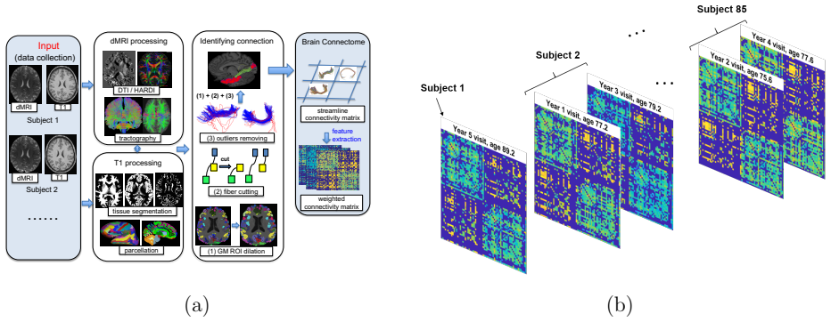
Modern neuroimaging technologies, combined with state-of-the-art data processing pipelines, have made it possible to collect longitudinal observations of an individual's brain connectome at different ages. It is of substantial scientific interest to study how brain connectivity varies over time in relation to human cognitive traits. In brain connectomics, the structural brain network for an individual corresponds to a set of interconnections among brain regions. We propose a symmetric bilinear logistic regression to learn a set of small subgraphs relevant to a binary outcome from longitudinal brain networks as well as estimating the time effects of the subgraphs. We enforce the extracted signal subgraphs to have clique structure which has appealing interpretations as they can be related to neurological circuits. The time effect of each signal subgraph reflects how its predictive effect on the outcome varies over time, which may improve our understanding of interactions between the aging of brain structure and neurological disorders. Application of this method on longitudinal brain connectomics and cognitive capacity data shows interesting discovery of relevant interconnections among a small set of brain regions in frontal and temporal lobes with better predictive performance than competitors.

Figures

Figures reproduced from arXiv: 1908.05627 by the authors.

**Figure 2.** Average computational time (in seconds) per iteration for 30 runs versus the [PITH_FULL_IMAGE:figures/full_fig_p016_2.png] view at source ↗

**Figure 3.** Average computational time (in seconds) per iteration (left) and average peak [PITH_FULL_IMAGE:figures/full_fig_p017_3.png] view at source ↗

Figures from the paper (12 more)

**Figure 4.** Figure 4: The 3D array Xi constructed for each subject i in a tensor regression. Then the nonzero entries in each component matrix β (h) 1 ◦ β (h) 2 = β (h) 1 β (h)> 2 are supposed to locate an outcome-relevant subgraph. However, the partial symmetry in Xi when fixing the 3rd d…

**Figure 5.** Figure 5: Overlay of 11 basis subgraphs corresponding to [PITH_FULL_IMAGE:figures/full_fig_p019_5.png]

**Figure 6.** Figure 6: True coefficient matrix βhβ > h for h = 1 (upper) and h = 2 (lower) in a simulated dataset, along with the corresponding signal subgraphs (middle) and age effects {λh(g)} (right). where β1 = q3 , β2 = q11 in (32), and the functions {λh(g) : h = 1, 2} are set as the rig…

**Figure 7.** Figure 7: Mean deviances of SBLR 5-fold cross validation (CV) on simulated data. The grid [PITH_FULL_IMAGE:figures/full_fig_p021_7.png]

**Figure 8.** Figure 8: Estimated results of SBLR under K = 5 where the penalty factors are chosen by the one-standard-error rule. Left: the estimated nonzero component matrix β3β > 3 ; the matrix is normalized such that the off-diagonal element with the largest magnitude is 1. Middle: the co…

**Figure 9.** Figure 9: Profiles of estimated entries in coefficient matrices [PITH_FULL_IMAGE:figures/full_fig_p023_9.png]

**Figure 10.** Figure 10: Estimated results of unstructured logistic regression (28) with elastic-net penalty [PITH_FULL_IMAGE:figures/full_fig_p024_10.png]

**Figure 11.** Figure 11: Estimated results of NSTR model (29) - (31) under [PITH_FULL_IMAGE:figures/full_fig_p025_11.png]

**Figure 12.** Figure 12: Estimated results of SBLR on a simulated dataset with [PITH_FULL_IMAGE:figures/full_fig_p026_12.png]

**Figure 13.** Figure 13: Selected connections predictive of supernormals from LR with constant (left), [PITH_FULL_IMAGE:figures/full_fig_p028_13.png]

**Figure 14.** Figure 14: Left: the selected signal subgraph corresponding to the nonzero component [PITH_FULL_IMAGE:figures/full_fig_p029_14.png]

**Figure 15.** Figure 15: Left: the selected signal subgraph corresponding to the nonzero component [PITH_FULL_IMAGE:figures/full_fig_p030_15.png]

Discussion (0). Continue with ORCID to comment.

Reference graph

Works this paper leans on

26 extracted references · 21 canonical work pages

[1]

I., Cohen, A

Casey, B., Cannonier, T., Conley, M. I., Cohen, A. O., Barch, D. M., Heitzeg, M. M., Soules, M. E., Teslovich, T., Dellarco, D. V., Garavan, H., et al. (2018). The adolescent brain cognitive development ( ABCD ) study: imaging acquisition across 21 sites. Developmental Cognitive Neuroscience

work page 2018
[2]

M., Fischl, B., and Sereno, M

Dale, A. M., Fischl, B., and Sereno, M. I. (1999). Cortical surface-based analysis: I. segmentation and surface reconstruction. Neuroimage , 9(2):179--194

work page 1999
[3]

S., S \'e gonne, F., Fischl, B., Quinn, B

Desikan, R. S., S \'e gonne, F., Fischl, B., Quinn, B. T., Dickerson, B. C., Blacker, D., Buckner, R. L., Dale, A. M., Maguire, R. P., Hyman, B. T., Albert, M. S., and Killiany, R. J. (2006). An automated labeling system for subdividing the human cerebral cortex on MRI scans into gyral based regions of interest. NeuroImage , 31(3):968 -- 980

work page 2006
[4]

and Li, R

Fan, J. and Li, R. (2001). Variable selection via nonconcave penalized likelihood and its oracle properties. Journal of the American Statistical Association , 96(456):1348--1360

2001
[5]

H., van der Kouwe, A

Fischl, B., Salat, D. H., van der Kouwe, A. J., Makris, N., S \'e gonne, F., Quinn, B. T., and Dale, A. M. (2004). Sequence-independent segmentation of magnetic resonance images. NeuroImage , 23(Supplement 1):S69 -- S84

work page 2004
[6]

Friedman, J., Hastie, T., and Tibshirani, R. (2010). Regularization paths for generalized linear models via coordinate descent. Journal of Statistical Software , 33(1):1--22

2010
[7]

Girard, G., Whittingstall, K., Deriche, R., and Descoteaux, M. (2014). Towards quantitative connectivity analysis: reducing tractography biases. NeuroImage , 98:266 -- 278

work page 2014
[8]

R., Bernstein, M

Jack Jr, C. R., Bernstein, M. A., Fox, N. C., Thompson, P., Alexander, G., Harvey, D., Borowski, B., Britson, P. J., L. Whitwell, J., Ward, C., et al. (2008). The A lzheimer's disease neuroimaging initiative (adni): Mri methods. Journal of Magnetic Resonance Imaging: An Official Journal of the International Society for Magnetic Resonance in Medicine , 27(...

work page 2008

Show all 26 references

[9]

L., Reid, R

Jin, Y., Huang, C., Daianu, M., Zhan, L., Dennis, E. L., Reid, R. I., Jack Jr, C. R., Zhu, H., Thompson, P. M., and Initiative, A. D. N. (2017). 3d tract-specific local and global analysis of white matter integrity in A lzheimer's disease. Human Brain Mapping , 38(3):1191--1207

2017
[10]

M., Littlefield, A

King, K. M., Littlefield, A. K., McCabe, C. J., Mills, K. L., Flournoy, J., and Chassin, L. (2018). Longitudinal modeling in developmental neuroimaging research: Common challenges, and solutions from developmental psychology. Developmental Cognitive Neuroscience , 33:54--72

2018
[11]

Kolda, T. G. and Bader, B. W. (2009). Tensor decompositions and applications. SIAM review , 51(3):455--500

2009
[12]

F., Susmaras, T., Caughlin, B

Kraus, M. F., Susmaras, T., Caughlin, B. P., Walker, C. J., Sweeney, J. A., and Little, D. M. (2007). White matter integrity and cognition in chronic traumatic brain injury: a diffusion tensor imaging study. Brain , 130(10):2508--2519

2007
[13]

L., Sambataro, F., Verchinski, B

Lemaitre, H., Goldman, A. L., Sambataro, F., Verchinski, B. A., Meyer-Lindenberg, A., Weinberger, D. R., and Mattay, V. S. (2012). Normal age-related brain morphometric changes: nonuniformity across cortical thickness, surface area and gray matter volume? Neurobiology of Aging...

2012
[14]

P., Porsteinsson, A., Baran, T

Lin, F., Ren, P., Mapstone, M., Meyers, S. P., Porsteinsson, A., Baran, T. M., Initiative, A. D. N., et al. (2017). The cingulate cortex of older adults with excellent memory capacity. Cortex , 86:83--92

2017
[15]

H., Neher, P

Maier-Hein, K. H., Neher, P. F., Houde, J.-C., C \^o t \'e , M.-A., Garyfallidis, E., Zhong, J., Chamberland, M., Yeh, F.-C., Lin, Y.-C., Ji, Q., et al. (2017). The challenge of mapping the human connectome based on diffusion tractography. Nature Communications , 8(1):1349

2017
[16]

A., Cheema, A

Mapstone, M., Lin, F., Nalls, M. A., Cheema, A. K., Singleton, A. B., Fiandaca, M. S., and Federoff, H. J. (2017). What success can teach us about failure: the plasma metabolome of older adults with superior memory and lessons for A lzheimer's disease. Neurobiology of Aging , ...

2017
[17]

Park, D. C. and Reuter-Lorenz, P. (2009). The adaptive brain: aging and neurocognitive scaffolding. Annual Review of Psychology , 60:173--196

2009
[18]

Rodrigue, K. M. and Raz, N. (2004). Shrinkage of the entorhinal cortex over five years predicts memory performance in healthy adults. Journal of Neuroscience , 24(4):956--963

2004
[19]

J., Gefen, T., Shi, J., Samimi, M., Bigio, E., Weintraub, S., Geula, C., and Mesulam, M.-M

Rogalski, E. J., Gefen, T., Shi, J., Samimi, M., Bigio, E., Weintraub, S., Geula, C., and Mesulam, M.-M. (2013). Youthful memory capacity in old brains: anatomic and genetic clues from the northwestern superaging project. Journal of Cognitive Neuroscience , 25(1):29--36

2013
[20]

W., Stepanovic, M

Sun, F. W., Stepanovic, M. R., Andreano, J., Barrett, L. F., Touroutoglou, A., and Dickerson, B. C. (2016). Youthful brains in older adults: preserved neuroanatomy in the default mode and salience networks contributes to youthful memory in superaging. Journal of Neuroscience ,...

2016
[21]

Tibshirani, R. (1996). Regression shrinkage and selection via the lasso. Journal of the Royal Statistical Society. Series B (Statistical Methodology) , 58(1):267--288

1996
[22]

Wang, L., Zhang, Z., and Dunson, D. B. (2019). Symmetric bilinear regression for signal subgraph estimation. IEEE Transactions on Signal Processing , 67:1929--1940

2019
[23]

Zhang, Z., Descoteaux, M., Zhang, J., Girard, G., Chamberland, M., Dunson, D., Srivastava, A., and Zhu, H. (2018). Mapping population-based structural connectomes. Neuroimag , 172:130 -- 145

2018
[24]

and Li, L

Zhou, H. and Li, L. (2014). Regularized matrix regression. Journal of the Royal Statistical Society: Series B (Statistical Methodology) , 76(2):463--483

2014
[25]

Zhou, H., Li, L., and Zhu, H. (2013). Tensor regression with applications in neuroimaging data analysis. Journal of the American Statistical Association , 108(502):540--552

2013
[26]

and Hastie, T

Zou, H. and Hastie, T. (2005). Regularization and variable selection via the elastic net. Journal of the Royal Statistical Society: Series B (Statistical Methodology) , 67(2):301--320

2005

Pith tools

Reviewed August 14, 2026 · model on record in the stance chip above.

[1] [1]

I., Cohen, A

Casey, B., Cannonier, T., Conley, M. I., Cohen, A. O., Barch, D. M., Heitzeg, M. M., Soules, M. E., Teslovich, T., Dellarco, D. V., Garavan, H., et al. (2018). The adolescent brain cognitive development ( ABCD ) study: imaging acquisition across 21 sites. Developmental Cognitive Neuroscience

work page 2018

[2] [2]

M., Fischl, B., and Sereno, M

Dale, A. M., Fischl, B., and Sereno, M. I. (1999). Cortical surface-based analysis: I. segmentation and surface reconstruction. Neuroimage , 9(2):179--194

work page 1999

[3] [3]

S., S \'e gonne, F., Fischl, B., Quinn, B

Desikan, R. S., S \'e gonne, F., Fischl, B., Quinn, B. T., Dickerson, B. C., Blacker, D., Buckner, R. L., Dale, A. M., Maguire, R. P., Hyman, B. T., Albert, M. S., and Killiany, R. J. (2006). An automated labeling system for subdividing the human cerebral cortex on MRI scans into gyral based regions of interest. NeuroImage , 31(3):968 -- 980

work page 2006

[4] [4]

and Li, R

Fan, J. and Li, R. (2001). Variable selection via nonconcave penalized likelihood and its oracle properties. Journal of the American Statistical Association , 96(456):1348--1360

2001

[5] [5]

H., van der Kouwe, A

Fischl, B., Salat, D. H., van der Kouwe, A. J., Makris, N., S \'e gonne, F., Quinn, B. T., and Dale, A. M. (2004). Sequence-independent segmentation of magnetic resonance images. NeuroImage , 23(Supplement 1):S69 -- S84

work page 2004

[6] [6]

Friedman, J., Hastie, T., and Tibshirani, R. (2010). Regularization paths for generalized linear models via coordinate descent. Journal of Statistical Software , 33(1):1--22

2010

[7] [7]

Girard, G., Whittingstall, K., Deriche, R., and Descoteaux, M. (2014). Towards quantitative connectivity analysis: reducing tractography biases. NeuroImage , 98:266 -- 278

work page 2014

[8] [8]

R., Bernstein, M

Jack Jr, C. R., Bernstein, M. A., Fox, N. C., Thompson, P., Alexander, G., Harvey, D., Borowski, B., Britson, P. J., L. Whitwell, J., Ward, C., et al. (2008). The A lzheimer's disease neuroimaging initiative (adni): Mri methods. Journal of Magnetic Resonance Imaging: An Official Journal of the International Society for Magnetic Resonance in Medicine , 27(...

work page 2008