REVIEW 2 major objections 4 minor 66 references
Simulations of starspot anomalies within TESS exoplanetary transit light curves -- I. The detection limits of starspot anomalies in TESS light curves
T0 review · 2 major / 4 minor · reviewed 2026-08-14 · deepseek-v4-flash
Pith's one-line read Starspot anomalies will be observable in TESS 2-minute transit light curves, with detection limits of 4,900 ± 1,700 km for M4V, 13,800 ± 6,000 km for M1V, and 15,900 ± 6,800 km for K5V host stars.
desk verdict Solid TESS starspot detectability grid with a real factor-of-two flux normalization error in Eq. 7 and an overstated abstract; radius limits survive. read the letter →
The pith
A machine-rendered reading of the paper's core claim, the machinery that carries it, and where it could break.
The reading
What carries the argument
The central object is PRISM, a pixellation-based transit-starspot model that tiles the stellar disc into two-dimensional elements, assigns each element an intensity (with quadratic limb darkening and a blackbody-based spot contrast $\rho_\mathrm{spot}$), and integrates the received flux as the planet crosses. The load-bearing detection procedure compares the mean amplitude of the simulated spot anomaly, averaged over the in-transit data points that describe it, with the rms scatter of the light curve; a spot is counted as detected only when that mean exceeds $2.0\sigma$. This statistic, not the spot physics alone, sets every numerical limit, and it is the reason the paper finds a planet-size-dependent detection bias.
What would settle it
Inject starspot anomalies of the predicted threshold sizes into real TESS 2-minute light curves of active M4V, M1V, and K5V dwarfs, add the same Gaussian noise levels, and measure the recovery rate under the $2.0\sigma$ mean-amplitude rule; if recovery falls well below expectation, the claimed detection limits are optimistic. Conversely, a systematic search of TESS archival single transits that never finds blips at the predicted scales would falsify the observability conclusion.
Extended reading notes
Core claim
The central claim is that a starspot occulted by a transiting planet will produce a detectable brightening 'blip' in TESS 2-minute data for realistic M4V, M1V, and K5V hosts, with specific size limits. The authors define detection by the mean amplitude of the anomaly exceeding $2.0\sigma$ of the photometric noise within a single transit, and use this to derive $r_\mathrm{spot} = 0.045 \pm 0.016\,R_*$ for M4V, $0.040 \pm 0.017\,R_*$ for M1V, and $0.038 \pm 0.016\,R_*$ for K5V, corresponding to $4{,}900 \pm 1{,}700$ km, $13{,}800 \pm 6{,}000$ km, and $15{,}900 \pm 6{,}800$ km. Under the most favourable combinations (cool spots, 600 nm, 60 ppm noise), the smallest detected spot is $r_\mathrm{spot} = 0.017\,R_*$, or about 1,900 km on an M4V star. They also find a universal relation between the spot flux change $\Delta F_\mathrm{spot}$ and the planetary transit flux change $\Delta F_p$, with the minimum detectable $\Delta F_\mathrm{spot} = 0.00015 \pm 0.00001$ at $k = 0.082 \pm 0.004$. An additional result is the unexpected trend that small, hot spots are only detected by larger planets, which the authors attribute to the fixed 2-minute cadence and the mean-amplitude detection statistic.
Load-bearing premise
The results stand on the choice that a spot is 'detected' only when the mean amplitude of its in-transit blip exceeds $2.0\sigma$ of the photometric noise in a single transit; a different detection statistic or the use of phase-folded transits would move every reported limit.
Editorial extensions
If this is right
- Many TESS transit light curves of active K and M dwarfs will contain measurable starspot blips, so analyses of those systems should include transit-starspot modelling rather than treating the transit shape as spot-free.
- The quoted radius limits give a concrete target scale: spots larger than roughly 4,900 km on an M4V dwarf should generally be recoverable in single 2-minute transits, with the best-case floor near 1,900 km.
- The quadratic $\Delta F_\mathrm{spot}$–$\Delta F_p$ relation lets observers predict, for a given transit depth, the smallest spot flux deficit and lowest contrast that TESS can reveal, which can guide target selection for spot studies.
- Unmodelled spot anomalies can bias measured planetary radii, limb-darkening coefficients, and transit timings; the paper's detection limits therefore bracket the severity of this bias for TESS systems.
- Detectable single-transit spot anomalies enable the starspot-tracking technique for measuring stellar rotation and sky-projected spin-orbit obliquity in systems where the Rossiter-McLaughlin effect is impractical.
Reading between the lines
- An obvious extension the authors leave implicit is that a full likelihood-ratio or joint multi-transit analysis, rather than a single-transit mean-amplitude threshold, would likely push the effective detection limits somewhat smaller; their numbers should be read as conservative for dedicated analyses.
- The predicted abundance of detectable blips implies that archival TESS light curves can be mined for single-transit spot occultations; counting their occurrence as a function of stellar activity would test the underlying spot-coverage assumptions.
- The same simulation pipeline could be rerun for the 20-second cadence TESS mode, which should substantially improve the small-planet/small-hot-spot cases that the 2-minute cadence punishes.
- The $\Delta F_\mathrm{spot}$–$\Delta F_p$ relation could be turned into an estimator for spot contrast from a measured blip and known transit depth, effectively giving a spot-temperature diagnostic in the TESS band.
Signed reviews
Editorial analysis
A structured set of objections, weighed in public.
Referee Report
Summary. The manuscript presents a large grid of forward-model simulations, using the PRISM transit-starspot code, of starspot anomalies in TESS 2-minute-cadence transit light curves of M4V, M1V, and K5V host stars. A starspot is deemed detected when the mean amplitude of the anomaly, averaged over the in-transit points describing the blip, exceeds 2.0 sigma of the injected Gaussian photometric noise. The authors report per-scenario minimum detectable spot radii, global detection limits of 4900 +/- 1700 km (M4V), 13800 +/- 6000 km (M1V), and 15900 +/- 6800 km (K5V), and a fitted quadratic relation between the spot flux deficit and the planet transit depth (Eq. 9), from which they quote a minimum detectable DeltaF_spot = 0.00015 +/- 0.00001 at k = 0.082 +/- 0.004. The central qualitative conclusion is that starspot anomalies will be observable in many TESS 2-minute transit light curves of K and M dwarfs.
Significance. If the quantitative calibration is corrected, the paper is a useful, transparent reference point for the TESS community: it gives a concrete expectation that starspot 'blips' will appear in 2-minute-cadence transits, and it quantifies how the detectability depends on spot temperature, wavelength, noise, orbital period, and planet size. The strengths include a large and clearly described simulation grid, a forward model benchmarked against JKTEBOP to about 10 ppm, explicit model-recovery tests motivating the detection threshold, and the promise to release the simulated light curves. However, the flux-deficit normalization in Eq. (7) is incorrect by approximately a factor of two, which propagates into Eq. (9), Figs. 11-12, and the abstract's DeltaF_spot value; this is a load-bearing quantitative error, although the radius-based detection limits from the PRISM simulations themselves are not affected. The numeric limits also depend on the chosen 2-sigma mean-amplitude detection statistic. With those caveats, the broad conclusion that starspot anomalies will be observable in TESS transit light curves is defensible.
major comments (2)
- [Section 3.6, Table 4 and Eq. (9)] The definition of DeltaF_spot is normalized incorrectly. For a spot at the centre of the stellar disc occulted by a planet, the flux deficit relative to the unspotted disc is set by the spot's projected area on the sky, pi R*^2 sin^2(rspot), divided by the full stellar disc area pi R*^2, i.e. DeltaF_spot = sin^2(rspot)(1 - rho_spot). Equation (7) instead uses the spherical-cap area normalized by the hemisphere area, (1 - cos rspot)(1 - rho_spot). For the small angular radii used throughout the paper (rspot <= 0.35 rad), sin^2(rspot) ~ 2(1 - cos rspot), so every DeltaF_spot value, the fitted coefficients in Eq. (9), the abstract's headline DeltaF_spot = 0.00015 +/- 0.00001, and the Section 3.6 contrast-extrapolation examples are too low by roughly this factor. In particular, the example claiming that a rspot = 1 degree spot cannot be detected for a 1 R_Jup planet around a 1 R_sun star would likely be reversed under the correct normalization. The optimum location k = 0.082 is nearly unaffected because the factor is approximately constant across the fitted range, and the radius detection limits computed directly from PRISM are unaffected. The authors should recompute all flux-deficit results with the projected-area normalization.
- [Section 3, detection criterion] Section 3.6, Table 4 and Eq. (9): The conversion from per-scenario rspot limits to DeltaF_spot uses a single mean contrast, rho_bar_spot, per spectral class (Table 4) rather than the actual rho_spot for each of the 1296 scenarios. Because rspot and rho_spot are correlated in the simulations, the product of the means is not the mean of the products, which introduces a systematic bias in the DeltaF_spot points used to fit Eq. (9). When correcting Eq. (7), the authors should recompute Fig. 12 and Eq. (9) using the per-scenario rho_spot values, or demonstrate quantitatively that the averaging is unbiased.
minor comments (4)
- [Section 2.3] The number of M4V simulations is given as 6870 in Section 3.1 but 6718 in the Table A.1 caption; analogous discrepancies appear for M1V (7769 in the text vs. 7812 in Table A.2) and for K5V (5934 in the text vs. 6737 in Table A.3). These should be made consistent.
- [Section 2.3] The injected noise levels are described as the 'photometric sensitivity' of TESS; please clarify whether the 60-200 ppm values are point-to-point rms per 2-minute cadence sample, and how the cited 60 ppm hr^-1/2 noise floor is converted to the 2-minute cadence used in the simulations.
- [Section 3.6] Both DeltaF_p = k^2 and DeltaF_spot ignore limb darkening, even though PRISM applies quadratic limb darkening and the spot is placed at disc centre. For the limb-darkening coefficients used here, the centre-to-mean intensity ratio is about 1.15, which would alter the absolute flux-deficit values beyond the factor-of-two issue in Eq. (7); the approximations should be stated explicitly and ideally corrected.
- [Section 2.1] The use of three monochromatic wavelengths (600, 785, 1000 nm) to represent the TESS passband is a simplification, since rho_spot is wavelength-dependent and the TESS band is broad; a sentence quantifying the expected systematic uncertainty from not integrating over the full passband would be helpful.
Circularity Check
No significant circularity; simulations are forward models with independent benchmarking, and the one self-citation (PRISM) is not load-bearing.
full rationale
The paper's derivation chain is a forward simulation study: PRISM generates synthetic TESS transit light curves with known starspot parameters, noise is added, and the detection limit is the smallest input rspot whose mean anomaly amplitude exceeds the adopted 2.0-sigma threshold. The 2.0-sigma criterion is not a hidden fit to the conclusions; it is an explicit detection statistic justified by parameter-recovery tests described in Section 3. The only self-citation of consequence is PRISM itself (Tregloan-Reed et al. 2013, 2015, 2018), but PRISM is benchmarked against the independent JKTEBOP code (Section 2, average difference ~10 ppm) and has been used by other groups, so it qualifies as independent support under the rules rather than a load-bearing self-citation. The quadratic relation in Eq. 9 is an empirical fit to simulation outputs, not a derivation that assumes Eq. 9 or the abstract's minimum DeltaF_spot. The reviewer's hemisphere-area normalization concern about Eq. 7 is a quantitative correctness issue, not circularity, because it does not make any derived quantity identical to an input by construction. The stated unexpected trend is explicitly attributed to the cadence and mean-amplitude detection method, and is not presented as an independent prediction from an assumed conclusion. Overall, the central claims are self-contained conditional on the adopted detection metric.
Assumptions & free parameters
free parameters (4)
- Detection threshold for anomaly amplitude =
2.0 sigma (rms)
- Quadratic coefficient a in Eq. 9 =
0.00028 +/- 0.00001
- Quadratic coefficient b in Eq. 9 =
-0.00121 +/- 0.00001
- Quadratic coefficient c in Eq. 9 =
0.00147 +/- 0.00002
assumptions (7)
- domain assumption Starspot and photosphere radiate as blackbodies, so spot contrast rho_spot follows Eq. 2 (Silva 2003).
- domain assumption The transit and starspot signals are accurately modeled by PRISM's pixellation scheme with quadratic limb darkening.
- domain assumption Noise is white and Gaussian at 60, 100, 150, or 200 ppm rms with no red noise or systematics.
- domain assumption A starspot anomaly can generally be detected only in a single transit because stellar rotation moves the spot between transits.
- domain assumption The starspot is placed at the centre of the stellar disc to minimize foreshortening, giving the smallest detectable rspot.
- domain assumption The mean amplitude of the starspot anomaly, not the maximum, is the correct detection statistic.
- standard math Standard physics: Kepler's third law, solid angle formula, and Planck function.
Cite this review
Pith. "Pith review of Simulations of starspot anomalies within TESS exoplanetary transit light curves -- I. The detection limits of starspot anomalies in TESS light curves." pith.science (2026). https://pith.science/paper/JNCTBBEB
@misc{pith2026190805747,
  author       = {Pith},
  title        = {Pith review of: Simulations of starspot anomalies within TESS exoplanetary transit light curves -- I. The detection limits of starspot anomalies in TESS light curves},
  year         = {2026},
  howpublished = {\url{https://pith.science/paper/JNCTBBEB}},
  note         = {Machine review of arXiv:1908.05747}
}
abstract
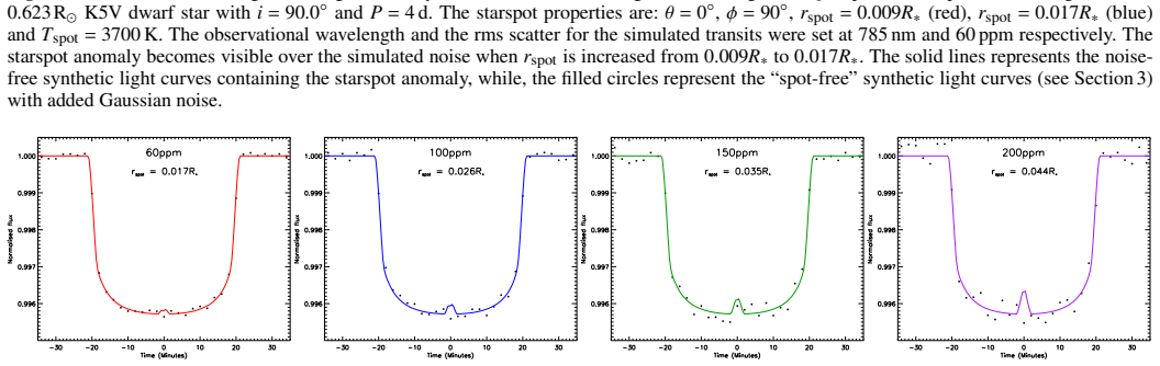
20573 simulations of planetary transits around spotted stars were conducted using the transit-starspot model, \texttt{PRISM}. In total 3888 different scenarios were considered using three different host star spectral types, M4V, M1V and K5V. The mean amplitude of the starspot anomaly was measured and compared to the photometric precision of the light curve, to determine if the starspot anomaly's characteristic "blip" was noticeable in the light curve. The simulations show that, starspot anomalies will be observable in TESS 2\,min cadence data. The smallest starspot detectable in TESS transit light curves has a radius of $\approx1900$\,km. The starspot detection limits for the three host stars are: $4900\pm1700$\,km (M4V), $13800\pm6000$\,km (M1V) and $15900\pm6800$\,km (K5V). The smallest change in flux of the starspot ($\Delta F_\mathrm{spot} = 0.00015\pm0.00001$) can be detected when the ratio between the planetary and stellar radii, $k = 0.082\pm0.004$. The results confirm known dependencies between the amplitude of the starspot anomaly and the photometric parameters of the light curve. The results allowed the characterisation of the relationship between the change in flux of the starspot anomaly and the change in flux of the planetary transit for TESS transit light curves.
Figures

Figures from the paper (9 more)




Reference graph
Works this paper leans on
-
[1]
Ballerini, P ., Micela, G., Lanza, A. F., & Pagano, I. 2012, A& A, 539, A140
work page 2012
-
[2]
Barnes, J. R., Je ffers, S. V ., Jones, H. R. A., et al. 2015, ApJ, 812, 42
work page 2015
-
[3]
2018, MNRAS, 4 75, 4467 Béky, B., Kipping, D
Bayliss, D., Gillen, E., Eigmüller, P ., et al. 2018, MNRAS, 4 75, 4467 Béky, B., Kipping, D. M., & Holman, M. J. 2014, MNRAS, 442, 368 6
work page 2018
-
[4]
J., Koch, D., Basri, G., et al
Borucki, W. J., Koch, D., Basri, G., et al. 2010, Science, 327 , 977
work page 2010
-
[5]
S., von Braun, K., van Belle, G., et al
Boyajian, T. S., von Braun, K., van Belle, G., et al. 2012, ApJ , 757, 112
work page 2012
-
[6]
Chen, G., Guenther, E. W., Pallé, E., et al. 2017, A&A, 600, A1 38
work page 2017
-
[7]
2017, A&A, 600, A30
Claret, A. 2017, A&A, 600, A30
2017
-
[8]
Dotter, A., Chaboyer, B., Jevremovi ´c, D., et al. 2008, ApJS, 178, 89
work page 2008
Show all 66 references
- [9]
-
[10]
Dressing, C. D. & Charbonneau, D. 2013, ApJ, 767, 95
2013
-
[11]
Dressing, C. D. & Charbonneau, D. 2015, ApJ, 807, 45
2015
-
[12]
J., Marley, M
Fortney, J. J., Marley, M. S., & Barnes, J. W. 2007, ApJ, 659, 1 661
2007
-
[13]
D., Bayliss, D., Brahm, R., et al
Hartman, J. D., Bayliss, D., Brahm, R., et al. 2015, AJ, 149, 1 66
2015
-
[14]
2016, A&A, 586, A131
Herrero, E., Ribas, I., Jordi, C., et al. 2016, A&A, 586, A131
2016
-
[15]
X., Burt, J., V anderburg, A., et al
Huang, C. X., Burt, J., V anderburg, A., et al. 2018, ApJ, 868, L39
2018
-
[16]
Jackson, R. J. & Je ffries, R. D. 2013, MNRAS, 431, 1883
2013
-
[17]
M., Twicken, J
Jenkins, J. M., Twicken, J. D., McCauli ff, S., et al. 2016, in Proc. SPIE, V ol. 9913, Software and Cyberinfrastructure for Astronomy IV , 99133E
2016
-
[18]
A., Gazak, J
Johnson, J. A., Gazak, J. Z., Apps, K., et al. 2012, AJ, 143, 11 1
2012
-
[19]
G., Lendl, M., Cubillos, P
Juvan, I. G., Lendl, M., Cubillos, P . E., et al. 2018, A&A, 610 , A15
2018
-
[20]
K., Ramirez, R., Kasting, J
Kopparapu, R. K., Ramirez, R., Kasting, J. F., et al. 2013, Ap J, 765, 131
2013
-
[21]
2013, MNRAS, 436, 2
Mancini, L., Ciceri, S., Chen, G., et al. 2013, MNRAS, 436, 2
2013
-
[22]
2015, A&A, 579, A136
Mancini, L., Esposito, M., Covino, E., et al. 2015, A&A, 579, A136
2015
-
[23]
2014, MNRAS, 443, 2391
Mancini, L., Southworth, J., Ciceri, S., et al. 2014, MNRAS, 443, 2391
2014
-
[24]
2017, MNRAS, 46 5, 843
Mancini, L., Southworth, J., Raia, G., et al. 2017, MNRAS, 46 5, 843
2017
-
[25]
Maxted, P . F. L. 2016, A&A, 591, A111
2016
-
[26]
McLaughlin, D. B. 1924, ApJ, 60, 22
1924
-
[27]
D., et al
Mohler-Fischer, M., Mancini, L., Hartman, J. D., et al. 2013 , A&A, 558, A55
2013
-
[28]
2014, MNRAS, 444, 1 721
Montalto, M., Boué, G., Oshagh, M., et al. 2014, MNRAS, 444, 1 721
2014
-
[29]
Morton, T. D. & Swift, J. 2014, ApJ, 791, 10
2014
-
[30]
J., et al
Nikolov, N., Chen, G., Fortney, J. J., et al. 2013, A&A, 553, A 26 O’Neal, D., Ne ff, J. E., Saar, S. H., & Cuntz, M. 2004, AJ, 128, 1802
2013
-
[31]
2013, A&A, 549, A35 Prša, A., Conroy, K
Oshagh, M., Boisse, I., Boué, G., et al. 2013, A&A, 549, A35 Prša, A., Conroy, K. E., Horvat, M., et al. 2016, ApJS, 227, 29 Prša, A. & Zwitter, T. 2005, ApJ, 628, 426
2013
-
[32]
A., et al
Rabus, M., Alonso, R., Belmonte, J. A., et al. 2009, A&A, 494, 391
2009
-
[33]
R., Latham, D
Ricker, G. R., Latham, D. W., V anderspek, R. K., et al. 2009, i n Bulletin of the American Astronomical Society, V ol. 41, American Astronomical Society Meeting Abstracts #213, 193
2009
-
[34]
R., Winn, J
Ricker, G. R., Winn, J. N., V anderspek, R., et al. 2014, in Spa ce Telescopes and Instrumentation 2014: Optical, Infrared, and Millimeter Wave, V ol. 9143, 914320
2014
-
[35]
R., Winn, J
Ricker, G. R., Winn, J. N., V anderspek, R., et al. 2015, Journ al of Astronomical
2015
-
[36]
Rossiter, R. A. 1924, ApJ, 60, 15
1924
-
[37]
C., Winn, J
Sanchis-Ojeda, R., Fabrycky, D. C., Winn, J. N., et al. 2012, Nature, 487, 449
2012
-
[38]
& Winn, J
Sanchis-Ojeda, R. & Winn, J. N. 2011, ApJ, 743, 61
2011
-
[39]
N., Holman, M
Sanchis-Ojeda, R., Winn, J. N., Holman, M. J., et al. 2011, Ap J, 733, 127
2011
-
[40]
N., Marcy, G
Sanchis-Ojeda, R., Winn, J. N., Marcy, G. W., et al. 2013, ApJ , 775, 54
2013
-
[41]
1910, Publications of the Allegheny Observ atory of the Univer- sity of Pittsburgh, 1, 123
Schlesinger, F. 1910, Publications of the Allegheny Observ atory of the Univer- sity of Pittsburgh, 1, 123
1910
-
[42]
1916, Publications of the Allegheny Observ atory of the Univer- sity of Pittsburgh, 3, 23
Schlesinger, F. 1916, Publications of the Allegheny Observ atory of the Univer- sity of Pittsburgh, 3, 23
1916
-
[43]
Silva, A. V . R. 2003, ApJ, 585, L147 Silva-Válio, A. 2010, in IAU Symposium, V ol. 264, IAU Sympos ium, ed. A. G
2003
-
[44]
Kosovichev, A. H. Andrei, & J.-P . Roelot, 440–442 Silva-V alio, A., Lanza, A. F., Alonso, R., & Barge, P . 2010, A&A, 510, A25
2010
-
[45]
2008, MNRAS, 386, 1644
Southworth, J. 2008, MNRAS, 386, 1644
2008
-
[46]
2010, MNRAS, 408, 1689
Southworth, J. 2010, MNRAS, 408, 1689
2010
-
[47]
2011, MNRAS, 417, 2166
Southworth, J. 2011, MNRAS, 417, 2166
2011
-
[48]
2013, A&A, 557, A119
Southworth, J. 2013, A&A, 557, A119
2013
-
[49]
Southworth, J., Bruntt, H., & Buzasi, D. L. 2007, A&A, 467, 12 15
2007
-
[50]
C., Dominik, M., et al
Southworth, J., Hinse, T. C., Dominik, M., et al. 2009, ApJ, 7 07, 167
2009
-
[51]
Southworth, J., Maxted, P . F. L., & Smalley, B. 2004, MNRAS, 3 51, 1277
2004
-
[52]
Southworth, J., Smalley, B., Maxted, P . F. L., Claret, A., & E tzel, P . B. 2005, MNRAS, 363, 529
2005
-
[53]
G., Oelkers, R
Stassun, K. G., Oelkers, R. J., Pepper, J., et al. 2018, AJ, 15 6, 102
2018
-
[54]
W., Winn, J
Sullivan, P . W., Winn, J. N., Berta-Thompson, Z. K., et al. 2015, ApJ, 809, 77
2015
-
[55]
W., Winn, J
Sullivan, P . W., Winn, J. N., Berta-Thompson, Z. K., et al. 2017, ApJ, 837, 99
2017
-
[56]
2015, MNRAS, 450, 1760
Tregloan-Reed, J., Southworth, J., Burgdorf, M., et al. 2015, MNRAS, 450, 1760
2015
-
[57]
2018 , MNRAS, 474, 5485
Tregloan-Reed, J., Southworth, J., Mancini, L., et al. 2018 , MNRAS, 474, 5485
2018
-
[58]
2013, MNRA S, 428, 3671 V alio, A., Estrela, R., Netto, Y ., Bravo, J
Tregloan-Reed, J., Southworth, J., & Tappert, C. 2013, MNRA S, 428, 3671 V alio, A., Estrela, R., Netto, Y ., Bravo, J. P ., & de Medeiros , J. R. 2017, ApJ, 835, 294 V anderspek, R., Huang, C. X., V anderburg, A., et al. 2019, ApJ, 871, L24
2013
-
[59]
2019, AJ, 157, 51
Wang, S., Jones, M., Shporer, A., et al. 2019, AJ, 157, 51
2019
-
[60]
J., Pollacco, D
Wheatley, P . J., Pollacco, D. L., Queloz, D., et al. 2013, in E uropean Physi- cal Journal Web of Conferences, V ol. 47, European Physical J ournal Web of Conferences, 13002
2013
-
[61]
Wilson, R. E. 1979, ApJ, 234, 1054
1979
-
[62]
Wilson, R. E. 1990, ApJ, 356, 613
1990
-
[63]
Wilson, R. E. 2008, ApJ, 672, 575
2008
-
[64]
Wilson, R. E. 2012, AJ, 144, 73
2012
-
[65]
Wilson, R. E. & Devinney, E. J. 1971, ApJ, 166, 605
1971
-
[66]
Winn, J. N. 2010, Exoplanet Transits and Occultations, ed. S . Seager (University of Arizona Press), 55–77 Article number, page 14 of 24 Tregloan-Reed , Unda-Sanzana: Simulations of starspot ano malies within TESS Appendix A: Full results of all simulations Article number, pag...
2010
Reviewed August 14, 2026 · model on record in the stance chip above.
Discussion (0). Continue with ORCID to comment.