REVIEW 3 major objections 4 minor 12 references
Generating Random Parameters in Feedforward Neural Networks with Random Hidden Nodes: Drawbacks of the Standard Method and How to Improve It
T0 review · 3 major / 4 minor · reviewed 2026-08-14 · deepseek-v4-flash
Pith's one-line read Placing each sigmoid's inflection point inside the input hypercube, via $b = -a^T x^*$, and drawing slope angles uniformly ($a = 4\tan\alpha$) improves random-hidden-node networks and cuts overfitting.
desk verdict A correct and simple bias-placement trick for random hidden nodes, with a new slope-angle parameterization, let down by a thin empirical evaluation and ambiguous hyperparameter selection. read the letter →
The pith
A machine-rendered reading of the paper's core claim, the machinery that carries it, and where it could break.
The reading
What carries the argument
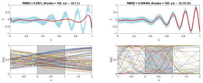
The carrying object is the sigmoid inflection point $\chi$, defined by $h(\chi)=0.5$, together with the identity $\tan\alpha = a/4$ between the weight $a$ and the slope angle $\alpha$ at that point. The standard method's deficiency is quantified by the distribution of $\chi = -b/a$: under uniform $a,b$, only a quarter of one-dimensional sigmoids have their steepest fragment inside the input interval, and the fraction inside the hypercube grows with dimension (roughly 46% for $n=2$ and above 90% for $n\ge 7$). The proposed method uses the bias rule $b=-a^T x^*$ with $x^* \in H$ (a random point of $H$, a random training point, or a cluster prototype) to move every inflection surface into the input hypercube, and uses $a=4\tan\alpha$ with uniform $\alpha$ to spread slope angles evenly.
What would settle it
Take a low-dimensional regression task and build two random-hidden-node sets with identical slope-angle distributions, one using $b=-a^T x^*$ with all $x^*$ inside $H$ and one adding a fixed large offset so all inflection surfaces miss $H$; if their test errors are nearly equal, the paper's premise that only in-cube inflection fragments contribute would be falsified.
Extended reading notes
Core claim
On the paper's own terms, the central discovery is that bias and weight play different roles in a random-hidden-node sigmoid and should therefore be generated differently. With standard draws $a,b \sim U(-u,u)$, the inflection point obeys $\chi = -b/a$, and the paper derives its density: $f(\chi)=1/4$ for $|\chi| < 1$ and $f(\chi)=1/(4\chi^2)$ for $|\chi| \ge 1$, so for one input only 25% of sigmoids have their steepest fragment in the unit interval. Choosing any $x^*$ inside the input domain and setting $b = -a^T x^*$ puts a sigmoid's inflection surface directly at $x^*$, so every hidden node can be made locally flexible where the target fluctuates. Independently, because the sigmoid's slope at its inflection point satisfies $\tan\alpha = a/4$, generating $\alpha \sim U(\alpha_{\min}, \alpha_{\max})$ and setting $a = 4\tan\alpha$ produces uniformly distributed slope angles, which the experiments link to reduced overfitting.
Load-bearing premise
The load-bearing premise is that only each sigmoid's steepest fragments around its inflection level $h=0.5$ are useful for modeling target-function nonlinearity, so saturated pieces inside the input cube cannot compensate; the simulations also presume that the tuning bounds $u$ or $\alpha_{\min}$ are chosen on validation data only, without leaking test information.
Editorial extensions
If this is right
- Standard uniform generation is wasteful in low-dimensional problems, where only about a quarter of sigmoids have their steepest fragments in the input interval; the proposed bias rule makes the useful fragment present for every node.
- Selecting $x^*$ as a random training point instead of a uniformly random point of $H$ distributes the hidden nodes according to data density, and selecting cluster prototypes gives a data-adaptive placement.
- Uniform slope angles from $U(\alpha_{\min}, \alpha_{\max})$ prevent the concentration of near-vertical sigmoids that occurs with wide uniform weight ranges, which the simulations associate with overfitting.
- In the reported experiments, the angle-based version $PM_\alpha$ attains the lowest mean test errors for $n=2,5,10$, and for $n=5$ and $n=10$ its error keeps decreasing as node count grows while the standard methods' error rises.
- For the single-variable target, the proposed method reached a similar RMSE with 35 hidden nodes while the standard method needed more than 60.
Reading between the lines
- The bias-placement rule should transfer to other sigmoidal or threshold-like activations, where one redefines $x^*$ as the point at which the activation passes through its central value and sets the shift accordingly.
- Uniform slope angles offer a principled regularisation dial: capping $\alpha_{\max}$ by the steepest slope the target function actually exhibits would replace the trial-and-error choice of $u$ with an interpretable geometric bound.
- Drawing $x^*$ from the most recent data would let random-hidden-node networks track nonstationary inputs without retraining output weights, a streaming adaptation the paper does not discuss.
- The paper's own probability calculation predicts that the improvement over standard generation should shrink as input dimension grows; testing the method on low-dimensional benchmarks is therefore the most discriminating next experiment.
Signed reviews
Editorial analysis
A structured set of objections, weighed in public.
Referee Report
Summary. The paper studies how random weights and biases are generated for single-hidden-layer feedforward neural networks with random hidden nodes (FNNRHN). It argues that the standard practice of drawing both weights and biases uniformly from the same interval [−u,u] is wasteful, because in low-dimensional problems most sigmoid inflection points fall outside the input hypercube H, leaving only saturated (nearly flat) fragments inside H. The proposed fix is to draw each bias as b = −a^T x^*, where x^* is a point in H (e.g., a random training point), which forces h(x^*) = 0.5 and hence places the inflection hyperplane of that sigmoid inside H (Section 2, Eq. (6)). The paper further proposes generating each weight as a = 4 tan α, where α is drawn uniformly from [α_min, α_max], in order to obtain hidden units with uniformly distributed slope angles (Section 3, Eq. (9)). Algorithm 1 combines these ideas. The empirical section compares the standard method (SM), the proposed bias-placement method (PMu), and the version with angle-uniform weights (PMα) on two synthetic target functions, Eq. (1) and Eq. (10), for dimensions n = 2, 5, 10, reporting test RMSE versus number of hidden nodes.
Significance. The mathematical core of the paper is mostly sound and useful. The derivation of the inflection-point density in Eq. (4) is correct for one-dimensional inputs, the bias rule in Eq. (6) is a simple and elegant construction that indeed guarantees a point of the inflection hyperplane inside H, and Eq. (9) is a clean parameter-free transformation from a slope angle to a weight. These are concrete, implementable tools that could help practitioners generate more informative random hidden units. The paper also provides a full algorithm and reproducible-looking simulation code. However, the significance of the empirical claim is currently limited. The two target functions are both strongly oscillatory, so they favor the paper's premise that only steep, inflection-centered fragments are useful; the absence of smoother targets makes the generality of the improvement unclear. In addition, the hyperparameter selection in Section 4 is not described precisely enough to rule out test-set leakage. If the authors address these evaluation issues, the contribution would be a useful practical guideline for randomized neural-network training.
major comments (3)
- [Section 2 (Eq. (6) and the discussion of saturated sigmoids)] The central improvement rests on the premise, stated in Section 2, that 'the saturated fragments of these sigmoids ... are useless for modeling nonlinear TFs.' This is a heuristic, not a theorem. A saturated sigmoid still has a nonzero derivative and can contribute a slowly varying or nearly constant component to a linear combination, which may be useful for smooth or low-frequency targets. The experiments use only the two oscillatory functions g(x) = sin(20 exp x) x^2 and its multivariate additive version, Eq. (10), so they cannot detect whether forcing all inflection hyperplanes into H helps on smoother targets or whether it reduces the diversity of the basis. I ask the authors to test the method on at least one smooth/low-frequency target and to provide either a quantitative argument for why saturated fragments are useless or a more nuanced statement of when Eq. (6) is expected to help.
- [Section 4, Figure 5 (hyperparameter selection)] The text says 'For each node number the optimal value of u or α_min was selected from u ∈ {1, 2, ..., 10, 20, 50, 100} and α_min ∈ {0°, 10°, ..., 80°}, respectively,' but it does not state whether this selection was made on the test set, a validation set, or by some other criterion. If the test set was used to choose the hyperparameters, the reported PMα curves are envelopes over a grid of hyperparameters and the improvement over SM may be substantially overstated. Please specify the selection procedure, and ideally report results for a fixed hyperparameter chosen by a proper validation split or via nested cross-validation.
- [Section 2, right panel of Figure 2 (multivariate inflection points)] For n > 1 the sigmoid h(x) = σ(a^T x + b) has an (n−1)-dimensional inflection hyperplane, not an isolated point, so the statement 'probability that χ belongs to H' as a function of n is conceptually unclear unless χ is defined as a random point on that hyperplane or as the vector of coordinate-wise ratios. The subsequent construction in Eq. (6) is clear, but the motivation via Figure 2 would benefit from an explicit definition of what is being plotted for n > 1.
minor comments (4)
- [Section 4, first paragraph and method definitions] Several equation references are incorrect: biases are set by Eq. (6), not Eq. (8), and in the definitions of PMu and PMα the biases are again said to follow Eq. (8) when they should follow Eq. (6). Please correct these cross-references.
- [Algorithm 1] The orientation of the output matrix A is not fully specified: the loop generates a_{i,j} with i indexing nodes and j indexing inputs, but the bias formula uses a_i^T x_i^*. Please clarify whether columns or rows of A correspond to hidden nodes, or use a consistent indexing convention.
- [Section 2, Eq. (4)] The derivation of f(χ) would be easier to follow if the support of χ and the change of variables b = −aχ were stated explicitly; in the current typesetting the integration limits for |χ| ≥ 1 are easy to misread.
- [Section 1] The abstract and introduction say the standard method draws weights and biases from 'the same fixed interval,' but the paper also cites work that optimizes u. Please clarify the scope of the critique so as not to conflate the fixed-interval choice with the wider class of tuned uniform methods.
Circularity Check
No material circularity: the bias and slope-angle constructions are explicit identities, and the self-citations are contextual.
full rationale
The paper's two central formulas are explicit constructions rather than hidden circular reductions. In Section 2, Eq. (6), b = -a^T x* is obtained by solving h(x*)=0.5, so the guarantee that the sigmoid's inflection point lies at x* is an algebraic identity, not a fitted parameter repackaged as a prediction. In Section 3, Eq. (8) defines the slope angle as alpha = arctan(a/4), and Eq. (9), a = 4 tan(alpha), is simply the inverse transformation; drawing alpha uniformly therefore produces uniformly distributed slope angles by construction. These are transparent design choices. The self-citations [10] and [11] appear in the introduction as context for recent developments and are not used to justify the derivations, the bias formula, or the experimental comparisons. The performance study selects u or alpha_min per node count from a grid without stating a validation split, which could overstate the reported improvements, but this is an experimental-model-selection concern rather than circularity. Similarly, the premise that saturated sigmoids are useless is a heuristic assumption about how hidden units contribute to the fit; it is a correctness or generality risk, not a circular reduction. Because the central claims are self-contained and the only self-citations are non-load-bearing, the circularity level is minimal.
Assumptions & free parameters
free parameters (4)
- u (weight bound) =
chosen per node count from {1, 2, ..., 10, 20, 50, 100}
- alpha_min (minimum slope angle) =
chosen from {0, 10, ..., 80} degrees
- alpha_max (maximum slope angle) =
90 degrees in the experiments
- x* selection scheme =
not stated for experiments
assumptions (4)
- domain assumption FNNRHN with random parameters sampled from a symmetric interval has universal approximation capability.
- domain assumption A sigmoid is useful for modeling a target function only through its most nonlinear fragments around the inflection level h = 0.5; saturated fragments are useless.
- standard math In the standard method the weights and biases are independent uniform random variables on [-u,u].
- domain assumption For multidimensional inputs, the probability that a randomly generated sigmoid has an inflection point in H grows with dimension as plotted in Fig. 2.
Cite this review
Pith. "Pith review of Generating Random Parameters in Feedforward Neural Networks with Random Hidden Nodes: Drawbacks of the Standard Method and How to Improve It." pith.science (2026). https://pith.science/paper/NEMPHPYS
@misc{pith2026190805864,
  author       = {Pith},
  title        = {Pith review of: Generating Random Parameters in Feedforward Neural Networks with Random Hidden Nodes: Drawbacks of the Standard Method and How to Improve It},
  year         = {2026},
  howpublished = {\url{https://pith.science/paper/NEMPHPYS}},
  note         = {Machine review of arXiv:1908.05864}
}
read the original abstract
The standard method of generating random weights and biases in feedforward neural networks with random hidden nodes, selects them both from the uniform distribution over the same fixed interval. In this work, we show the drawbacks of this approach and propose a new method of generating random parameters. This method ensures the most nonlinear fragments of sigmoids, which are most useful in modeling target function nonlinearity, are kept in the input hypercube. In addition, we show how to generate activation functions with uniformly distributed slope angles.
Figures


Figures from the paper (2 more)


Reference graph
Works this paper leans on
-
[1]
J. Principe, B. Chen, Universal approximation with convex optimiz ation: gimmick or reality?, IEEE Computational Intelligence Magazine 10 (2) (2015) 68–77. doi:10.1109/MCI.2015.2405352
arXiv 2015
-
[2]
D. Husmeier, Random vector functional link (R VFL) networks, in : Neu- ral Networks for Conditional Probability Estimation: Forecasting B e- yond Point Predictions, Springer-Verlag London, 1999, Ch. 6, pp. 87–97. doi:10.1007/978-1-4471-0847-4_6
-
[3]
L. Zhang, P. Suganthan, A survey of randomized algorithms for train- ing neural networks, Information Sciences 364–365 (2016) 146– 155. doi:10.1016/j.ins.2016.01.039
-
[4]
W. Cao, X. Wang, Z. Ming, J. Gao, A review on neural net- works with random weights, Neurocomputing 275 (2018) 278–287. doi:10.1016/j.neucom.2017.08.040. 8
-
[5]
S. Scardapane, D. Comminiello, M. Scarpiniti, A. Uncini, A semi- supervised random vector functional-link network based on the tr ans- ductive framework, Information Sciences 364-365 (2016) 156–1 66. doi:10.1016/j.ins.2015.07.060
-
[6]
D. Wang, M. Li, Stochastic configuration networks: Fundament als and algorithms, IEEE Transactions on Cybernetics 47 (10) (2017) 346 6–3479. doi:10.1109/TCYB.2017.2734043
arXiv 2017
-
[7]
M. Li, D. Wang, Insights into randomized algorithms for neural ne tworks: Practical issues and common pitfalls, Information Sciences 382–38 3 (2017) 170–178. doi:10.1016/j.ins.2016.12.007
-
[8]
L. Zhang, P. Suganthan, A comprehensive evaluation of random vector functional link networks, Information Sciences 367–368 (2016) 1 094–1105. doi:10.1016/j.ins.2015.09.025
Show all 12 references
-
[9]
F. Cao, D. Wang, H. Zhu, Y. Wang, An iterative learning algorithm f or feedforward neural networks with random weights, Information Sciences 328 (2016) 546–557. doi:10.1016/j.ins.2015.09.002
2016 doi
-
[10]
Dudek, Generating random weights and biases in feedforwar d neural networks with random hidden nodes, Information Sciences 481 (20 19) 33–
G. Dudek, Generating random weights and biases in feedforwar d neural networks with random hidden nodes, Information Sciences 481 (20 19) 33–
-
[11]
Dudek, Improving randomized learning of feedforward neur al networks by appropriate generation of random parameters, in: Advances in Compu- tational Intelligence
G. Dudek, Improving randomized learning of feedforward neur al networks by appropriate generation of random parameters, in: Advances in Compu- tational Intelligence. IW ANN 2019, Vol. 11506 of LNCS, Springer, 2 019, pp. 517–530. doi:10.1007/978-3-030-20521-8_43 . 9
2019 doi
-
[56]
doi:10.1016/j.ins.2018.12.063
2018 doi
Reviewed August 14, 2026 · model on record in the stance chip above.
Discussion (0). Continue with ORCID to comment.