Hermite interpolation and data processing errors on Riemannian matrix manifolds

Ralf Zimmermann

REVIEW 2 major objections 4 minor 39 references

Hermite interpolation and data processing errors on Riemannian matrix manifolds

T0 review · 2 major / 4 minor · reviewed 2026-08-14 · deepseek-v4-flash

Challenge this review Re-run · record.json Download PDF Read on arXiv ↗ Review JSON

Pith's one-line read A single tangent-space curve solves Hermite interpolation on any Riemannian manifold carrying exponential and logarithm maps.

desk verdict Sound Hermite construction, but the 'error bounds' are asymptotic heuristics and the numerical comparison skips existing Hermite methods. read the letter →

arxiv 1908.05875 v2 pith:IE6FMOMQ submitted 2019-08-16 math.NA cs.NA

Ralf Zimmermann This is my paper · ORCID

classification math.NAcs.NA MSC 15A1615B1033B3033F0553-0465F60

keywords HermiteinterpolationRiemannianmanifoldsStiefelmanifoldlogarithmsectionalcurvaturematrixSVDQRdecomposition

verification ladder T0 review T1 audit T2 compute T3 formal

The pith

A machine-rendered reading of the paper's core claim, the machinery that carries it, and where it could break.

The reading

This paper claims that Hermite interpolation of manifold-valued data need not be approached as a variational or control-point problem: if the manifold has computable Riemannian exponential and logarithm maps, a single tangent-space formula built from the classical cubic Hermite polynomials yields a $C^1$ curve through sampled points with sampled velocities. The author proves this as Theorem 2.1 and gives a concrete recipe for the one nontrivial ingredient, the differential of the logarithm map, which can be approximated by central finite differences. The same normal-coordinate viewpoint yields a quantitative relation between the error made by processing data in the tangent space and the manifold's sectional curvature, stated as Theorem 3.1. Numerical tests on the Stiefel manifold, including interpolation of QR factors, SVD factors, and a parametric option-pricing model, show the method producing lower interpolation errors than geodesic and tangent-space RBF baselines, with fewer exponential and logarithm evaluations than comparable Hermite manifold methods.

What carries the argument

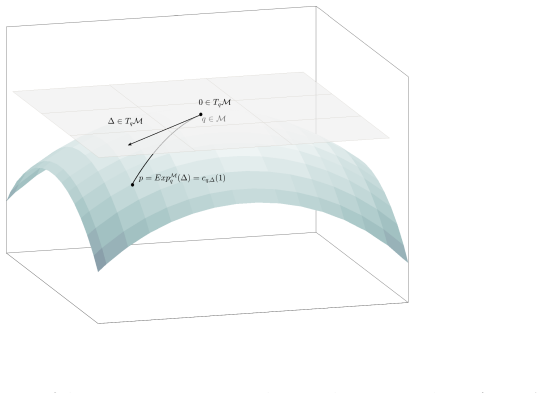
The load-bearing object is the Riemannian normal-coordinate chart centered at the terminal point $q$: the interpolating curve is the exponential image of a cubic Hermite curve $\gamma(t)=a_0(t)\Delta_p+b_0(t)\hat v_p+b_1(t)\hat v_q$ in $T_qM$. The only non-elementary ingredient is the push-forward of the start velocity through the logarithm transition map, $\hat v_p=d(\operatorname{Log}_q)_p(v_p)$, which the paper evaluates by central differences as $\big((\operatorname{Log}_q\circ\operatorname{Exp}_p)(hv_p)-(\operatorname{Log}_q\circ\operatorname{Exp}_p)(-hv_p)\big)/(2h)$; for the Stiefel manifold the paper derives an explicit formula for the derivative of the exponential via a block-matrix identity for the derivative of the matrix exponential. The curvature error bound is carried by the Jacobi-field expansion of $d(\operatorname{Exp}_q)_{\delta w}(\delta w^\perp)$, which is exactly the mechanism that turns tangent-space errors into manifold distances.

What would settle it

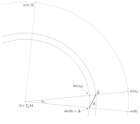
On a sphere, choose two tangent vectors $\Delta,\tilde\Delta$ at a point $q$ with small angle $s_0$ and norms $\delta,\tilde\delta<1$, compute the endpoints via the exponential map, and measure their geodesic distance; the inequality (3.1) predicts a specific shortening relative to the flat tangent-space distance, so a measured lengthening beyond the $O(s_0^2)$ term would refute the curvature relation.

Watch

Extended reading notes

Core claim

The central discovery is that a curve of the form $$c(t)=\operatorname{Exp}_q\big(a_0(t)\Delta_p+b_0(t)\hat v_p+b_1(t)\hat v_q\big)$$ with $\Delta_p=\operatorname{Log}_q(p)$, $\hat v_p=d(\operatorname{Log}_q)_p(v_p)$, and $\hat v_q=v_q$ solves the Hermite interpolation problem $c(t_0)=p$, $c(t_1)=q$, $\dot c(t_0)=v_p$, $\dot c(t_1)=v_q$ on any Riemannian manifold, provided $p$ and $q$ are not conjugate and the logarithm is defined. The proof works by expressing the whole curve in normal coordinates centered at the endpoint $q$, where the endpoint condition is automatic and the start condition becomes a single application of the differential of the logarithm. A second result relates the manifold distance between two exponential images of nearby tangent vectors to their tangent-space distance, with a first-order correction $\delta s_0\big(1-\tfrac{K_q(\sigma)}6\delta^2+o(\delta^2)\big)$ determined by the sectional curvature $K_q(\sigma)$: positive curvature shortens the propagated error, negative curvature amplifies it.

Load-bearing premise

The whole construction depends on consecutive sample points being close enough on the curved space that the map pulling one point back to the other's tangent space exists and that a small-step numerical derivative of that map is accurate.

Editorial extensions

If this is right

The method transfers to any Riemannian manifold with computable exponential and logarithm maps, including manifolds that carry no Lie-group, homogeneous-space, or symmetric-space structure.
Composite interpolation over many sample points is globally $C^1$ by construction, because each local arc ends with exactly the velocity that the next arc starts with.
Constructing the full curve costs $3k$ logarithm and $2k$ exponential evaluations for $k$ intervals, and each evaluation of the final curve costs one exponential evaluation, which is below the cost of the composite Bezier alternatives the paper compares against.
The same normal-coordinate machinery derives explicit manifold error bounds for any data-processing scheme that maps data to a tangent space, processes it there, and maps back to the manifold.
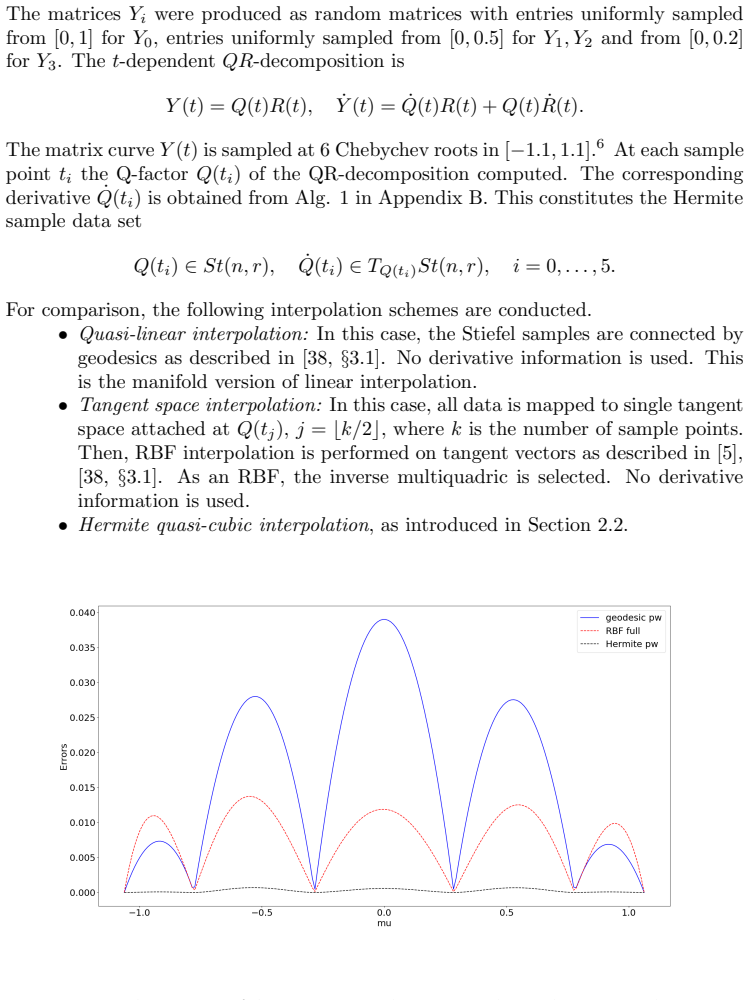
On the Stiefel manifold, the method interpolates the factors of QR and SVD decompositions with smaller relative Frobenius errors than geodesic or tangent-space RBF interpolation in the reported experiments.

Reading between the lines

Editorial extensions of the paper, not claims the author makes directly.

Because the local curve is anchored in normal coordinates at the right endpoint, swapping the endpoints changes the interpolant; an adaptive choice of anchor, for instance the endpoint with the larger remaining step, could reduce the chance that the logarithm fails, an effect the paper only observes numerically.
The curvature bound suggests an operational rule not stated by the author: on manifolds of positive sectional curvature, small tangent-space processing errors shrink on the manifold, so cheaper approximations such as retractions in place of exponentials may be safe; this could be tested by repeating the Stiefel experiments with retraction-based derivative transport.
The same transition-map derivative can in principle be computed to any order in the step size $h$ by higher-order finite differences or by differentiating the logarithm algorithm itself, which would remove the $O(h^2)$ error in the endpoint velocity without changing the interpolation formula.

Share X Bluesky LinkedIn Reddit HN

Signed reviews

No signed human review yet.

Editorial analysis

A structured set of objections, weighed in public.

Desk editor's note, referee report, and a circularity audit.

Desk Editor's Note

read the letter

Two things you should know. First, the Hermite interpolation construction in Theorem 2.1 is mathematically sound and practically useful: it transfers derivative samples through the differential of the log map, then builds a cubic Hermite curve in a single tangent space. The cost count (one log plus two logs/two exps per subinterval) is genuinely lower than the Bezier-based alternatives. Second, the advertised 'general error bounds' are not bounds. Theorem 3.1 is an asymptotic expansion with o(delta^2) and O(s0^2) remainders and no explicit constants; you cannot evaluate or certify it for a given manifold. The abstract overstates this.

What is new: the Log-differential transport in Theorem 2.1 and the explicit directional derivative of the Stiefel exponential in Lemma 4.1 (via the block matrix exponential trick) are real additions. The paper also works out the QR and SVD derivative bookkeeping cleanly. The numerical experiments on Stiefel show Hermite interpolation beating quasi-linear and RBF tangent-space interpolation by a wide margin, and the positive-curvature heuristic from Section 3 is consistent with the observed manifold errors being slightly smaller than tangent-space errors.

Soft spots: (1) As said, Theorem 3.1 is a qualitative curvature heuristic, not a bound. That should be fixed in the abstract and conclusions. (2) The numerical section does not compare with existing Hermite manifold methods (e.g., the blended-arc approaches of Jakubiak et al. or Gousenbourger et al.); the 'lower cost' claim is argued analytically but not demonstrated experimentally. (3) No code or data is released, so the numbers are not independently reproducible. (4) The Stiefel log algorithm used is the author's own (Zimmermann 2017), but that is a legitimate computational tool and the paper does not reduce to it; the main framework is independent. (5) The non-conjugate assumption and injectivity-radius caveat are stated, and Section 5.4 honestly shows the log failing for distant samples.

Verdict: this is a solid, useful paper for anyone doing manifold-valued interpolation with derivative data, especially on Stiefel/orthogonal-matrix problems. It deserves peer review; it needs a revised abstract and ideally a direct comparison with prior Hermite methods. I would send it to a knowledgeable referee.

Referee Report

2 major / 4 minor

Summary. The paper proposes a Riemannian generalization of local cubic Hermite interpolation. Given two sample points p, q and tangent vectors v_p, v_q on a Riemannian manifold, the method maps the data into the tangent space T_qM via the Riemannian logarithm, constructs the ordinary Euclidean cubic Hermite polynomial in that tangent space using the basis functions a0, b0, b1, and maps the result back to the manifold via the exponential map. The endpoint velocity at q is automatic, while the velocity at p is matched by transporting v_p through the differential d(Log_q)_p. The paper proves this construction in Theorem 2.1, discusses the practical finite-difference approximation of d(Log_q)_p, compares the computational effort with Bézier-type methods, and then derives an asymptotic relation between data-processing errors in normal coordinates and the sectional curvature of the manifold (Theorem 3.1). The numerical part specializes the framework to the compact Stiefel manifold, including formulas for differentiating the Stiefel exponential via Mathias' theorem, and presents experiments for the QR decomposition, low-rank SVD interpolation, and a Black-Scholes option-pricing application.

Significance. The Hermite construction is elementary, geometrically natural, and potentially useful: it applies to any Riemannian manifold for which exp and log algorithms are available, and the explicit Stiefel derivative formula in Lemma 4.1 is a concrete computational contribution. The numerical experiments are relevant and cover nontrivial applications. The paper also openly identifies its main practical constraint, namely that consecutive samples must lie close enough for the Stiefel logarithm to converge. The curvature-error relation in Theorem 3.1 is conceptually attractive and gives a clean qualitative explanation of why the manifold errors in the Stiefel experiments are slightly smaller than the tangent-space errors. However, as written the theorem is an asymptotic expansion, not a computable error bound; this is the main gap between the abstract's claims and the actual result. The central Hermite derivation is sound, and the overclaim is local and fixable, so the appropriate outcome is a major revision rather than rejection.

major comments (2)

[Abstract; Theorem 3.1, Eq. (3.1)] The abstract states that the paper 'provides general error bounds for manifold data processing methods', but Theorem 3.1 is an asymptotic estimate rather than a bound in the usual numerical-analysis sense. The right-hand side of Eq. (3.1) contains the unquantified terms o(δ^2) and O(s0^2), and the hypotheses δ, δ~<1 do not by themselves control these remainders; no explicit smallness condition involving the curvature or the injectivity radius is given. Consequently, for a fixed manifold with large sectional curvature, the displayed inequality cannot be evaluated or certified as a worst-case bound. Section 5.3 uses only the sign of the Stiefel curvature, not the quantitative content of the theorem. I recommend replacing 'general error bounds' by 'asymptotic error estimates' throughout, or alternatively adding explicit constants and a sufficient smallness condition under which the estimate is a true inequality with a computable remainder.
[Section 2.2, Eq. (2.11); Section 5.1] Theorem 2.1 is proved for the exact choice v_hat_p = d(Log_q)_p(v_p), but the general implementation described in Section 2.2 replaces this differential by the central finite-difference approximation in Eq. (2.11). The paper does not provide an error analysis showing how the O(h^2) truncation error and the convergence threshold of the iterative Stiefel logarithm affect the satisfaction of the Hermite conditions (1.2) or the C^1 assembly in Remark 1. The table in Section 5.1 gives empirical reconstruction errors for h = 10^-2 through 10^-7, but no theoretical statement links h to the interpolation error. Since the claimed generality is 'only exp and log algorithms are needed', the manuscript should either include a clear statement that the implemented curve satisfies the Hermite conditions only up to O(h^2) plus solver tolerance, or provide an explicit error estimate for the finite-difference step.

minor comments (4)

[Section 5.2 and Section 5.3] The figure numbering is inconsistent: the error curves in Section 5.2 are first introduced as Fig. 5.1 and then referenced as Fig. 5.2, and Section 5.3 again labels a plot as Fig. 5.2. Please renumber the figures and check all cross-references.
[Section 5.4] The section title refers to 'left singular values', but the experiment interpolates the left singular vectors U(μ); please adjust the title or the wording.
[Theorem 3.1] The notation σ = span(Δ, Δ~) assumes that Δ and Δ~ span a two-plane; when the two vectors are collinear, the sectional curvature K_q(σ) is not defined. Please add a convention for the collinear case or handle s0 = 0 separately.
[Remark 2(i)] The relation ε ≥ δ‖w(0)-w(s0)‖ and the subsequent bound δs0 ≤ 2δ arcsin(ε/(2δ)) are used to pass to Eq. (3.5), but Eq. (3.5) is only an asymptotic replacement for the exact angle-dependent expression; please state explicitly that the equality there is valid up to O(ε^2).

Circularity Check

0 steps flagged · score 0.0 of 10

No circularity: the Hermite construction is an explicit existence proof and the curvature estimate is a standard Jacobi-field expansion, not a fit.

full rationale

The central derivation (Theorem 2.1) constructs the interpolant explicitly: the auxiliary vector is defined by the inverse-function identity vhat_p = d(Log_q)_p(v_p), and the endpoint derivative then satisfies d(Exp_q)_{Delta_p}(vhat_p) = v_p because d(Log_q)_p is the inverse of d(Exp_q)_{Delta_p}. This is an existence/construction argument, not a fitted or renamed input. The curvature estimate (Theorem 3.1) is a Taylor expansion of the transition map Log_p o Exp_q along a circular arc, using the standard Jacobi-field estimate from do Carmo; it contains no fitted constants and is not derived from the Hermite ansatz. The paper's self-citations ([37] Stiefel logarithm, [38] manifold interpolation background) are used as computational tools and comparison baselines: [37] is an algorithm reproduced in Appendix D with stated assumptions, and the proof of Theorem 2.1 and Theorem 3.1 does not depend on it. The only notable caveat is a rigor/limitation issue, not circularity: Theorem 3.1 is an asymptotic expansion with o(delta^2) and O(s0^2) remainders, so the abstract's phrase 'general error bounds' overstates what is proved, and the conclusions admit that the main practical constraint is that consecutive samples must be close enough for the Stiefel logarithm to be well-defined. These are correctness and applicability observations, and they do not make the derivation circular.

Assumptions & free parameters 1 free parameters · 7 assumptions · 0 invented entities

The central construction relies on standard Riemannian geometry results (exponential map differential, Jacobi fields, injectivity radius) and on domain-specific tools for the Stiefel manifold (canonical metric, known exponential formula, curvature bounds, QR/SVD differentiation). All are cited from the literature; no ad hoc entities or fitted constants are introduced, apart from a numerical finite-difference step.

free parameters (1)

finite difference step h = 1e-4
Step size for central difference approximation (2.11) of d(Log_q)_p(v_p); selected from the error table in Section 5.1 as the best compromise, not fitted to the interpolation results.

assumptions (7)

standard math d(Exp_p)_0 = id, i.e., the exponential map differential at the origin is the identity.
Used to show ˙c(t1) = v_q in Theorem 2.1; cited from do Carmo §3, Prop. 2.9.
domain assumption The sample points p and q are not conjugate along the connecting geodesic.
Ensures d(Log_q)_p exists and equation (2.4) is invertible; stated as assumption in Theorem 2.1.
standard math Jacobi field asymptotic: ||J(t)|| = t - (K/6)t^3 + o(t^3) along a unit-speed geodesic.
The core of Theorem 3.1's error estimate; cited from do Carmo §5, Cor. 2.9 and 2.10.
domain assumption All data lies within the injectivity radius of the center q.
Required for Riemannian normal coordinates to be one-to-one; stated in Section 2.2 and used throughout the error analysis.
domain assumption The Stiefel exponential is given by the formula (4.2) with the canonical metric.
Background from Edelman, Arias, Smith (1998); used in Section 4 for the Stiefel tests.
domain assumption Stiefel sectional curvature is bounded by 0 ≤ K ≤ 5/4.
Invoked in Section 4 and 5.3 to explain the observed positive-curvature error behavior; from Rentmeesters (2013).
domain assumption The QR decomposition and SVD of the sampled matrix curves are differentiable.
Necessary for computing derivative samples in the experiments; QR from Walter, Lehmann, Lamour (2012), SVD from Hay et al. (2009).

how reviews work

0 comments

Cite this review

Pith. "Pith review of Hermite interpolation and data processing errors on Riemannian matrix manifolds." pith.science (2026). https://pith.science/paper/IE6FMOMQ

@misc{pith2026190805875,
  author       = {Pith},
  title        = {Pith review of: Hermite interpolation and data processing errors on Riemannian matrix manifolds},
  year         = {2026},
  howpublished = {\url{https://pith.science/paper/IE6FMOMQ}},
  note         = {Machine review of arXiv:1908.05875}
}

read the original abstract

The main contribution of this paper is twofold: On the one hand, a general framework for performing Hermite interpolation on Riemannian manifolds is presented. The method is applicable, if algorithms for the associated Riemannian exponential and logarithm mappings are available. This includes many of the matrix manifolds that arise in practical Riemannian computing application such as data analysis and signal processing, computer vision and image processing, structured matrix optimization problems and model reduction. On the other hand, we expose a natural relation between data processing errors and the sectional curvature of the manifold in question. This provides general error bounds for manifold data processing methods that rely on Riemannian normal coordinates. Numerical experiments are conducted for the compact Stiefel manifold of rectangular column-orthogonal matrices. As use cases, we compute Hermite interpolation curves for orthogonal matrix factorizations such as the singular value decomposition and the QR-decomposition.

Figures

Figures reproduced from arXiv: 1908.05875 by the authors.

**Figure 2.** [PITH_FULL_IMAGE:figures/full_fig_p006_2.png] view at source ↗

**Figure 3.** , where the outer dashed circular arc indicates the unit circle and the solid [PITH_FULL_IMAGE:figures/full_fig_p009_3.png] view at source ↗

Figures from the paper (7 more)

**Figure 5.** Figure 5 [PITH_FULL_IMAGE:figures/full_fig_p015_5.png]

**Figure 5.** Figure 5: displays the error curves for the quasi-linear and the quasi-cubic Hermite [PITH_FULL_IMAGE:figures/full_fig_p017_5.png]

**Figure 5.** Figure 5 [PITH_FULL_IMAGE:figures/full_fig_p018_5.png]

**Figure 5.6.** Figure 5.6: According to the figure, the tangent space interpolation method fails to [PITH_FULL_IMAGE:figures/full_fig_p018_5_6.png]

**Figure 5.** Figure 5 [PITH_FULL_IMAGE:figures/full_fig_p019_5.png]

**Figure 5.** Figure 5 [PITH_FULL_IMAGE:figures/full_fig_p020_5.png]

**Figure 5.** Figure 5 [PITH_FULL_IMAGE:figures/full_fig_p021_5.png]

Discussion (0). Continue with ORCID to comment.

Reference graph

Works this paper leans on

39 extracted references · 36 canonical work pages

[1]

Absil, P.-Y

P.-A. Absil, P.-Y. Gousenbourger, P. Striewski, and B. Wirth. Diﬀerentiable piecewise-B´ ezier surfaces on Riemannian manifolds. SIAM Journal on Imaging Sciences , 9(4):1788–1828, 2016. 25 Algorithm 4 Stiefel logarithm Input: base point U∈St(n,p ) and ˜U∈St(n,p ) ‘close’ to base point, τ >0 conver- gence threshold 1: M :=UT ˜U∈ Rp×p 2: QN := ˜U−UM∈ Rn×p #...

work page 2016
[2]

Absil, R

P.-A. Absil, R. Mahony, and R. Sepulchre. Optimization Algorithms on Matrix Manifolds . Princeton University Press, Princeton, New Jersey, 2008

work page 2008
[3]

Alekseevsky, A

D. Alekseevsky, A. Kriegl, P. W. Michor, and M. Losik. Choosing roots of polynomials smoothly. Israel Journal of Mathematics , 105(1):203–233, 1998

work page 1998
[4]

Amsallem

D. Amsallem. Interpolation on Manifolds of CFD-based Fluid and Finite Element-based Struc- tural Reduced-order Models for On-line Aeroelastic Prediction. PhD thesis, Stanford Uni- versity, 2010

work page 2010
[5]

Amsallem and C

D. Amsallem and C. Farhat. Interpolation method for adapting reduced-order models and application to aeroelasticity. AIAA Journal, 46(7):1803–1813, 2008

work page 2008
[6]

Bartels, J.C

R.H. Bartels, J.C. Beatty, and B.A. Barsky. An Introduction to Splines for Use in Computer Graphics and Geometric Modeling . Morgan Kaufmann Series in Comp. Elsevier Science, 1995

work page 1995
[7]

R. Bhatia. Matrix Analysis. Number 169 in Graduate Texts in Mathematics. Springer-Verlag, New York – Berlin – Heidelberg, 1997

work page 1997
[8]

Black and M

F. Black and M. Scholes. The pricing of options and corporate liabilities. J. Polit. Econ. , 81(3):637–654, 1973

work page 1973

Show all 39 references

[9]

Boumal and P.-A

N. Boumal and P.-A. Absil. A discrete regression method on manifolds and its application to data on SO(n). IFAC Proceedings Volumes, 44(1):2284 – 2289, 2011. 18th IFAC World Congress

2011
[10]

Bunse-Gerstner, R

A. Bunse-Gerstner, R. Byers, V. Mehrmann, and N. K. Nichols. Numerical computation of an analytic singular value decomposition of a matrix valued function.Numerische Mathematik, 60(1):1–39, 1991

1991
[11]

Camarinha, F

M. Camarinha, F. Silva Leite, and P. Crouch. On the geometry of riemannian cubic polynomials. Diﬀerential Geometry and its Applications , 15(2):107 – 135, 2001

2001
[12]

Crouch and F

P. Crouch and F. Silva Leite. The dynamic interpolation problem: On Riemannian manifolds, Lie groups, and symmetric spaces. Journal of Dynamical and Control Systems , 1(2):177– 202, 1995

1995
[13]

M. P. do Carmo. Riemannian Geometry. Mathematics: Theory & Applications. Birkh¨ auser Boston, 1992

1992
[14]

Edelman, T

A. Edelman, T. A. Arias, and S. T. Smith. The geometry of algorithms with orthogonality constraints. SIAM Journal on Matrix Analysis and Applications , 20(2):303–353, April 1998

1998
[15]

Oliphant, P

E.Jones, T. Oliphant, P. Peterson, et al. SciPy: Open source scientiﬁc tools for Python, 2001–. [Online; accessed July 2019

2001
[16]

Gousenbourger, E

P.-Y. Gousenbourger, E. Massart, and P.-A. Absil. Data ﬁtting on manifolds with composite 26 B´ ezier-like curves and blended cubic splines.Journal of Mathematical Imaging and Vision , online:1–27, 2018

2018
[17]

B. C. Hall. Lie Groups, Lie Algebras, and representations: An elementary introduction . Springer Graduate texts in Mathematics. Springer–Verlag, New York – Berlin – Heidel- berg, 2nd edition, 2015

2015
[18]

A. Hay, J. T. Borggaard, and D. Pelletier. Local improvements to reduced-order models using sensitivity analysis of the proper orthogonal decomposition. Journal of Fluid Mechanics , 629:41–72, 2009

2009
[19]

N. J. Higham. Functions of Matrices: Theory and Computation . Society for Industrial and Applied Mathematics, Philadelphia, PA, USA, 2008

2008
[20]

Hohmann and P

A. Hohmann and P. Deuﬂhard. Numerical Analysis in Modern Scientiﬁc Computing: An Introduction. Texts in Applied Mathematics. Springer New York, 2003

2003
[21]

Jakubiak, F

J. Jakubiak, F. S. Leite, and R. Rodrigues. A two-step algorithm of smooth spline generation on riemannian manifolds. Journal of Computational and Applied Mathematics , 194:177–191, 2006

2006
[22]

H.Le K. R. Kim, I. L. Dryden. Smoothing splines on riemannian manifolds, with applications to 3D shape space. arXiv:1801.04978v2, 2018

2018 arXiv
[23]

K. A. Krakowski, L. Machado, F. Silva Leite, and J. Batista. Solving interpolation prob- lems on Stiefel manifolds using quasi-geodesics. In Pr´ e-Publica¸ ci˜ oes do Departamento de Matem´ atica, number 15–36, Universidade de Coimbra, 2015

2015
[24]

J. M. Lee. Riemannian Manifolds: an Introduction to Curvature . Springer Verlag, New York – Berlin – Heidelberg, 1997

1997
[25]

J. M. Lee. Introduction to Smooth Manifolds . Graduate Texts in Mathematics. Springer New York, 2012

2012
[26]

Narcowich

F. Narcowich. Generalized Hermite interpolation and positive deﬁnite kernels on a Riemannian manifold. Journal of Mathematical Analysis and Applications , 190:165–193, 1995

1995
[27]

Nava-Yazdani and K

E. Nava-Yazdani and K. Polthier. De Casteljau’s algorithm on manifolds. Computer Aided Geometric Design, 30(7):722–732, 2013

2013
[28]

Noakes, G

L. Noakes, G. Heinzinger, and B. Paden. Cubic splines on curved spaces. IMA Journal of Mathematical Control and Information , 6(4):465–473, 12 1989

1989
[29]

Popiel and L

T. Popiel and L. Noakes. B´ ezier curves and C2 interpolation in Riemannian manifolds.Journal of Approximation Theory, 148(2):111–127, 2007

2007
[30]

Rentmeesters

Q. Rentmeesters. Algorithms for data ﬁtting on some common homogeneous spaces . PhD thesis, Universit´ e Catholique de Louvain, Louvain, Belgium, 2013

2013
[31]

Samir, P.-A

C. Samir, P.-A. Absil, A. Srivastava, and E. Klassen. A gradient-descent method for curve ﬁtting on Riemannian manifolds. Foundations of Computational Mathematics , 12(1):49– 73, Feb 2012

2012
[32]

Samir and I

C. Samir and I. Adouani. C1 interpolating B´ ezier path on Riemannian manifolds, with appli- cations to 3D shape space. Applied Mathematics and Computation , 348:371 – 384, 2019

2019
[33]

Steinke, M

F. Steinke, M. Hein, J. Peters, and B. Schoelkopf. Manifold-valued Thin-Plate Splines with Applications in Computer Graphics. Computer Graphics Forum, 2008

2008
[34]

S. F. Walter, L. Lehmann, and R. Lamour. On evaluating higher-order derivatives of the QR decomposition of tall matrices with full column rank in forward and reverse mode algorithmic diﬀerentiation. Optimization Methods and Software , 27(2):391–403, 2012

2012
[35]

Wen and W

Z. Wen and W. Yin. A feasible method for optimization with orthogonality constraints. Math- ematical Programming, 142(1):397–434, Dec 2013

2013
[36]

Zimmermann

R. Zimmermann. On the maximum likelihood training of gradient-enhanced spatial Gaussian processes. SIAM Journal on Scientiﬁc Computing , 35(6):A2554–A2574, 2013

2013
[37]

Zimmermann

R. Zimmermann. A matrix-algebraic algorithm for the Riemannian logarithm on the Stiefel manifold under the canonical metric. SIAM Journal on Matrix Analysis and Applications , 38(2):322–342, 2017

2017
[38]

Zimmermann

R. Zimmermann. Manifold interpolation and model reduction. arXiv:1902.06502v1, 2019

1902 arXiv
[39]

Zimmermann and K

R. Zimmermann and K. Debrabant. Parametric model reduction via interpolating orthonormal bases. In F. A. Radu, K. Kumar, I. Berre, D. N. Nordbotten, and I. S. Pop, editors, Nu- merical Mathematics and Advanced Applications ENUMATH 2017. Springer International Publishing, Cham,...

2017

Pith tools

Reviewed August 14, 2026 · model on record in the stance chip above.

[1] [1]

Absil, P.-Y

P.-A. Absil, P.-Y. Gousenbourger, P. Striewski, and B. Wirth. Diﬀerentiable piecewise-B´ ezier surfaces on Riemannian manifolds. SIAM Journal on Imaging Sciences , 9(4):1788–1828, 2016. 25 Algorithm 4 Stiefel logarithm Input: base point U∈St(n,p ) and ˜U∈St(n,p ) ‘close’ to base point, τ >0 conver- gence threshold 1: M :=UT ˜U∈ Rp×p 2: QN := ˜U−UM∈ Rn×p #...

work page 2016

[2] [2]

Absil, R

P.-A. Absil, R. Mahony, and R. Sepulchre. Optimization Algorithms on Matrix Manifolds . Princeton University Press, Princeton, New Jersey, 2008

work page 2008

[3] [3]

Alekseevsky, A

D. Alekseevsky, A. Kriegl, P. W. Michor, and M. Losik. Choosing roots of polynomials smoothly. Israel Journal of Mathematics , 105(1):203–233, 1998

work page 1998

[4] [4]

Amsallem

D. Amsallem. Interpolation on Manifolds of CFD-based Fluid and Finite Element-based Struc- tural Reduced-order Models for On-line Aeroelastic Prediction. PhD thesis, Stanford Uni- versity, 2010

work page 2010

[5] [5]

Amsallem and C

D. Amsallem and C. Farhat. Interpolation method for adapting reduced-order models and application to aeroelasticity. AIAA Journal, 46(7):1803–1813, 2008

work page 2008

[6] [6]

Bartels, J.C

R.H. Bartels, J.C. Beatty, and B.A. Barsky. An Introduction to Splines for Use in Computer Graphics and Geometric Modeling . Morgan Kaufmann Series in Comp. Elsevier Science, 1995

work page 1995

[7] [7]

R. Bhatia. Matrix Analysis. Number 169 in Graduate Texts in Mathematics. Springer-Verlag, New York – Berlin – Heidelberg, 1997

work page 1997

[8] [8]

Black and M

F. Black and M. Scholes. The pricing of options and corporate liabilities. J. Polit. Econ. , 81(3):637–654, 1973

work page 1973