Matrix Lie Maps and Neural Networks for Solving Differential Equations

Andrei Ivanov; Sergei Andrianov

REVIEW 4 major objections 6 minor 25 references

Matrix Lie Maps and Neural Networks for Solving Differential Equations

T0 review · 4 major / 6 minor · reviewed 2026-08-14 · deepseek-v4-flash

Challenge this review Re-run · record.json Download PDF Read on arXiv ↗ Review JSON

Pith's one-line read For polynomial ODE systems, a polynomial neural network with weights computed directly from the equation implements a matrix Lie map and approximates the general solution without training.

desk verdict A genuinely useful reframing of polynomial networks as truncated matrix Lie maps, with reproducible code, but the experiments never directly measure one-step map error, so the central claim is under-validated. read the letter →

arxiv 1908.06088 v1 pith:MIFJ2TIS submitted 2019-08-16 cs.NE cs.NAmath.DSmath.NAphysics.comp-ph

Andrei Ivanov , Sergei Andrianov This is my paper · ORCID

classification cs.NEcs.NAmath.DSmath.NAphysics.comp-ph MSC 34A3465L0568T07

keywords polynomialneuralnetworksmatrixLiemapsKroneckerpowersVanderPoloscillatorBurgers'equationdata-drivensystemidentificationdifferentialequations

verification ladder T0 review T1 audit T2 compute T3 formal

The pith

A machine-rendered reading of the paper's core claim, the machinery that carries it, and where it could break.

The reading

The core claim is that for ODE systems with polynomial or Taylor-expandable right-hand sides, the evolution map can be represented as a polynomial in the initial state, and this polynomial is exactly what a polynomial neural network computes. When the equation is known, the network's weight matrices are not learned; they are obtained directly by integrating a matrix recurrence derived from the Lie-transform formalism. The same built network then serves as a simulator for any initial condition inside the convergence region, so it need not be retrained or re-solved when initial conditions change. When the equation is unknown, the same architecture can be fitted from time-series data, and the Van der Pol example shows a network trained on one trajectory generalizing to new starting points. A Burgers' equation example extends the idea to PDEs by first reducing the PDE to a semi-discrete system of ODEs.

What carries the argument

The central object is the matrix Lie map: the evolution operator of the ODE system written as an infinite polynomial series in Kronecker powers of the initial state, $X(t|t_0) = M(t|t_0)\circ X_0 = \sum_{k\ge0} M_{1k} X_0^{[k]}$, where $X^{[k]}$ is the $k$-fold tensor product of the state vector with itself. The identity that carries the argument is the block recurrence $\frac{d}{dt}M_{ik}=\sum_{j=i}^{k}P_{ij}M_{jk}$, with block-diagonal initial conditions, which yields the weight matrices $W_i=M_{1i}$ once the $P_{ij}$ matrices from the polynomial expansion of the right-hand side are known. The network architecture, parallel layers that form Kronecker powers of the input and sum weighted outputs, is an evaluation circuit for this truncated propagator. In data-driven mode the same circuit becomes a model class whose weights are fitted from state transitions, so the Lie-map structure serves as an inductive bias instead of a derived object.

What would settle it

One decisive check: for a polynomial ODE with a known exact solution and a time step larger than the series convergence radius, compute the seventh-order weights from the recurrence and compare one-step predictions with the exact values; if the error does not shrink with increasing order or diverges, the convergence premise fails. A second check for Burgers: compare the semi-discrete 2000-ODE solution with the exact PDE solution on the same 1000-node mesh; if the difference is close to the reported $5.5\times10^{-3}$ MSE, the spatial discretization, not the Lie map, sets the reported accuracy.

Watch

Extended reading notes

Core claim

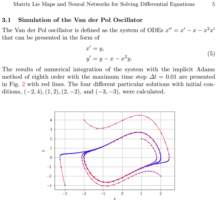
The central discovery is the identification of the polynomial neural network map $Y = W_0 + W_1 X + W_2 X^{[2]} + \cdots + W_k X^{[k]}$ with the truncated matrix Lie map of the differential equation. For a system written as $\frac{d}{dt}X = \sum_{k\ge0} P^1_k(t) X^{[k]}$, the weight matrices $W_i$ are the blocks $M_{1i}$ of the Lie transform, computed from the recurrence $\frac{d}{dt}M_{ik} = \sum_{j=i}^{k} P_{ij}M_{jk}$ with initial blocks $M_{kk}(t_0)=I^{[k]}$. This makes the network a propagator derived from the equation rather than an approximator fitted to solutions: once the weights are computed for a time step, the same map advances every state in the convergence region. For data-driven problems the same polynomial form is fitted to a time series; the Van der Pol experiment trains on one trajectory and reports mean relative errors around $10^{-5}$ on new initial conditions. For Burgers' equation the PDE is semi-discretized into a 2000-dimensional ODE system, and the resulting Lie-map network uses a time step five times larger than the benchmark finite-difference method while reporting lower mean squared error and less elapsed time.

Load-bearing premise

The load-bearing premise is that the truncated polynomial Lie-map series converges to the true solution over the chosen time step; for the Burgers example, an additional load-bearing premise is that the finite-difference spatial semi-discretization accurately represents the PDE, since the paper does not quantify that spatial error.

Editorial extensions

If this is right

For a known polynomial system, a simulator is obtained without training and without a numerical ODE solver: compute the weights once from the block recurrence, then iterate the polynomial map.
One network covers all initial conditions in the convergence region; the Van der Pol fits from a single trajectory and produces mean relative errors around $10^{-5}$ for new starting points.
Accuracy improves with truncation order: the Van der Pol tests report mean relative errors of $1.1\times10^{-2}$, $4\times10^{-4}$, and $4.7\times10^{-6}$ for third-, fifth-, and seventh-order maps.
For PDEs, the same method applies after semi-discretization; the Burgers example uses a time step five times larger than the benchmark finite-difference scheme and reports lower MSE ($5.5\times10^{-3}$ vs $8.0\times10^{-2}$) and lower elapsed time ($0.016$ s vs $0.055$ s).
For unknown equations, the same architecture can be fitted directly to time-series data, providing a data-driven model that generalizes to new initial conditions without an assumed analytic form.

Reading between the lines

Editorial extensions of the paper, not claims the author makes directly.

If the convergence assumption holds beyond the tested examples, the same construction could act as a coarse propagator for stiff or multiscale systems, since the map is a function of the time step rather than a local discretization; this regime is not examined in the paper.
For Burgers' equation, the reported MSE conflates Lie-map truncation error with the error of the finite-difference spatial semi-discretization; a clean separation would compare the semi-discrete ODE solution against the exact PDE solution on the same 1000-node mesh.
The data-driven mode's generalization likely depends on how well one trajectory covers the relevant state space; multi-stable or chaotic systems would require training data that visits the needed regions, an issue the paper lists as open for further research.

Share X Bluesky LinkedIn Reddit HN

Signed reviews

No signed human review yet.

Editorial analysis

A structured set of objections, weighed in public.

Desk editor's note, referee report, and a circularity audit.

Desk Editor's Note

read the letter

Worth a look if you work on surrogate models for ODEs. The new thing here is not the mathematics—matrix Lie maps are old—but the explicit identification with polynomial neural networks, which gives you a way to set the weights straight from the polynomial ODE and skip training. That is a real, useful observation, and the paper ships Keras notebooks that reproduce the Van der Pol and Burgers examples. Credit where due: the direct weight computation from equation (3) is standard and clearly explained, and the data-driven Van der Pol test generalizes to initial conditions outside the training set. That's a legitimate out-of-sample check.

The soft spots are real, and the stress-test note lands. The paper reports only integrated trajectory errors over ten time units, never the single-step map error. Since the Van der Pol oscillator is dissipative, a trajectory that converges to the limit cycle can look fine even if the one-step map is off. The missing step-size dependence study and the absence of a convergence-region bound matter. The paper leans on self-cited convergence theory [13,17]; the derivation of the weights is solid, but the truncation error is essentially taken on faith for the examples. The Burgers section is weaker: the PDE-to-ODE conversion is heuristic, the spatial discretization error is never quantified, and the comparison is against a first-order FDM with a smaller time step, so the accuracy and speed claims are not controlled. The performance statement in the conclusion leans on self-cited accelerator papers [24,25].

None of this kills the central identification. For a known polynomial ODE, the weight computation is exact up to truncation order, and that is useful. But the paper overstates what the experiments establish. The efficiency claim and the general-solution approximation need the one-step error and a controlled benchmark before they carry weight.

Who gets value: anyone building training-free surrogates for polynomial ODEs, or interpretable data-driven polynomial maps. It deserves a serious referee, but the referee should insist on stronger validation. My advice: engage with it, but treat the numerical claims as unproven until the single-step map and error bounds are actually reported.

Referee Report

4 major / 6 minor

Summary. The manuscript proposes a class of polynomial neural networks whose output is a truncated matrix Lie map (Eq. (4)). For polynomial ODE systems of the form (1), the authors argue that the network weights can be computed directly from the equation via Eq. (3), so that the network approximates the flow map and can be reused for arbitrary initial conditions without retraining. The same architecture is then applied in a data-driven mode, fitting weights from a single observed trajectory. The approach is demonstrated on the Van der Pol oscillator (Section 3) and on Burgers' equation (Section 4), where the PDE is first reduced to a system of ODEs by a finite-difference semi-discretization. The paper concludes that the Lie-map network can outperform traditional step-by-step numerical integration in accuracy and runtime.

Significance. If the central claim is correct, the construction is appealing: for polynomial ODEs, the map weights W_i = M_1i are derived from the equation rather than fitted, the network represents a genuine map rather than a particular solution, and the same computed or trained network can predict dynamics for new initial conditions. The paper also provides reproducible code (Section 5) and tests the data-driven version on initial conditions not seen in training. However, the reported experiments do not yet establish the load-bearing claim: the single-step error of the truncated Lie map is never measured, the convergence region is not characterized, and the Burgers example mixes an unquantified spatial-discretization error with the Lie-map truncation error. The contribution is therefore plausible but currently under-supported.

major comments (4)

[§3.1, Eq. (4)] The accuracy of the Lie-map network is only reported as a mean relative error of the full trajectory over ten time units (0.0110, 0.0004, and 4.7e-6 for third, fifth, and seventh orders). Because the Van der Pol oscillator is dissipative, trajectories from different initial conditions collapse to the same limit cycle, so trajectory-level agreement can be deceptively good even when the one-step map is inaccurate. The quantity that directly tests the truncation of Eq. (2) is the one-step error ||W0 + W1 X + ... + Wk X[k] - X(Δt|X)||, and it is not reported. Please add the one-step error as a function of truncation order and Δt, and show its behavior over a range of initial conditions.
[§4.2, Eq. (8)] The PDE-to-ODE conversion in Eq. (8) is not a hyperbolic approximation of Burgers' equation: the right-hand side of Eq. (6) contains both a diffusive term ν u_xx and a convective term u u_x, and after spatial discretization the system for U becomes a method-of-lines semi-discretization rather than ODEs of the form (8) with f(x,U) alone. The paper does not analyze the spatial-truncation error of this semi-discretization, so the MSE of 5.5e-3 reported in Table 2 includes an unquantified component that is not attributable to the Lie map. A spatial-convergence study (varying Δx at fixed Δt and vice versa) is needed before any accuracy comparison with the FDM can be interpreted.
[§2, Eq. (2)] The central claim that Eq. (4) with weights W_i = M_1i approximates the general solution requires a uniform convergence statement for the truncated series (2) over a known region of initial conditions and for a fixed Δt. The only backing offered is Ref. [17], which is from the same group, and no convergence region or step-size bound is stated for the Van der Pol or Burgers examples. Please either provide a self-contained error bound or a precise statement of the needed theorem, or report an empirical convergence study in Δt and truncation order that maps the region where the one-step map is accurate.
[Table 2] The comparison in Table 2 is between the Lie-map network with Δt = 1.25e-3 on a 1000x500 mesh and a first-order upwind/Euler FDM with Δt = 2.5e-4 on a 1000x2000 mesh. This does not support the conclusion that the proposed method provides better accuracy with less computational time: the FDM is only first-order accurate, the elapsed times are given without hardware or implementation details, and no refinement study shows how either error scales. A comparison against a higher-order reference solution and a convergence table in both Δx and Δt would be needed.

minor comments (6)

[General] Please harmonize the terminology: the title and abstract use 'matrix Lie maps' while the body refers to 'matrix Lie transform'.
[Figures 3-5] Axis labels, legends, and color descriptions are missing or incomplete in several figures; please make the plots self-contained.
[§3.1-3.2] Please state precisely how the mean relative error is defined (norm, time interval, number of samples), and report per-trajectory errors for the new initial conditions rather than only a pooled mean.
[Table 2] Please specify the units of the elapsed time, the computing environment, and how the MSE is computed over the spatial grid at t = 0.5.
[§5] Please include a version or commit hash for the GitHub repository and list the dependencies needed to reproduce the reported numbers.
[§2.1] The matrices P_ij in Eq. (3) are said to be taken from Ref. [14] but are not defined in the paper; a short definition would make Section 2 self-contained.

Circularity Check

0 steps flagged · score 0.0 of 10

No significant circularity: weights are computed from the ODE by the Lie-map recurrence and validated against independent numerical and analytic benchmarks.

full rationale

The central derivation is not circular. Eq. (4) defines the network output as the truncated Lie map, and Eq. (3) supplies a parameter-free recurrence for the weight matrices from the given ODE (1); nothing is fitted to the target solution in the simulation mode. The Van der Pol simulation is checked against an independent eighth-order Adams integration (Section 3.1), and the data-driven example in Section 3.2 fits one trajectory and then reports errors for new initial conditions, an out-of-sample prediction rather than a renamed fit. The Burgers example computes the Lie-map weights from a semi-discretized ODE system and compares against the analytic solution via MSE at t = 0.5 (Section 4.2, Table 2), so the benchmark is external. The paper relies on prior work for convergence and accuracy theory, including self-citations [14,17], but it also cites the independent Dragt monograph [13] for the same Lie-map machinery; a self-citation alone, without an exhibited reduction of the target claim to its own input, is not circularity under the rules. Validation gaps, such as the absence of a direct one-step error report and the unquantified spatial discretization error for Burgers, are correctness concerns rather than circularity.

Assumptions & free parameters 4 free parameters · 4 assumptions · 0 invented entities

The contribution rests on standard but self-cited convergence theory, on user-chosen truncation order and time step, and on an imported spatial discretization from the Airbus benchmark. The directly-computed weights are a derivation, not a fit, so no free parameters are fitted to the results to make the claims work.

free parameters (4)

truncation order k = 3, 5, 7 (Van der Pol); 3 (Burgers)
The polynomial degree is chosen by the authors for each example; errors decrease with order but no adaptive criterion is provided.
time step Δt = 0.01 (Van der Pol); 1.25e-3 (Burgers)
Selected by hand; the Burgers step is five times the baseline FDM step, which confounds the comparison.
spatial discretization and mesh = 1000 grid points, upwind first-order nonlinear term, centered second-order diffusion
The semi-discretization of the PDE is imported from the Airbus benchmark [19]; its error is not analyzed in the paper.
network hyperparameters for data-driven fit = third order, Adamax optimizer
The order and optimizer are chosen without sensitivity analysis; no error bars are reported.

assumptions (4)

domain assumption The vector field F(t,X) can be expanded in a convergent Taylor series in X (equation (1)).
Restricts the method to polynomial or analytic vector fields; stated in Section 2.
domain assumption The truncated Lie map series converges over the used time step.
Convergence is cited to Refs [13,17] rather than proved for the examples; load-bearing because the map is applied repeatedly.
ad hoc to paper Burgers' equation can be approximated as a hyperbolic system to derive the ODE set (8).
Section 4.2 uses the method of characteristics on a viscous PDE; the validity of treating the diffusion term as part of f(x,U) is not justified.
ad hoc to paper In the data-driven example, the one-step transition is exactly a polynomial of degree 3.
The loss function (Section 3.2) assumes this functional form; the paper does not test whether higher or lower degrees change the conclusion.

how reviews work

0 comments

Cite this review

Pith. "Pith review of Matrix Lie Maps and Neural Networks for Solving Differential Equations." pith.science (2026). https://pith.science/paper/MIFJ2TIS

@misc{pith2026190806088,
  author       = {Pith},
  title        = {Pith review of: Matrix Lie Maps and Neural Networks for Solving Differential Equations},
  year         = {2026},
  howpublished = {\url{https://pith.science/paper/MIFJ2TIS}},
  note         = {Machine review of arXiv:1908.06088}
}

read the original abstract

The coincidence between polynomial neural networks and matrix Lie maps is discussed in the article. The matrix form of Lie transform is an approximation of the general solution of the nonlinear system of ordinary differential equations. It can be used for solving systems of differential equations more efficiently than traditional step-by-step numerical methods. Implementation of the Lie map as a polynomial neural network provides a tool for both simulation and data-driven identification of dynamical systems. If the differential equation is provided, training a neural network is unnecessary. The weights of the network can be directly calculated from the equation. On the other hand, for data-driven system learning, the weights can be fitted without any assumptions in view of differential equations. The proposed technique is discussed in the examples of both ordinary and partial differential equations. The building of a polynomial neural network that simulates the Van der Pol oscillator is discussed. For this example, we consider learning the dynamics from a single solution of the system. We also demonstrate the building of the neural network that describes the solution of Burgers' equation that is a fundamental partial differential equation.

Figures

Figures reproduced from arXiv: 1908.06088 by the authors.

**Figure 1.** Neural network representation of third order matrix Lie map. To fit a proposed neural network, the training data is presented as a multivariate time series (table 1) that describes the evolution of the state vector of the dynamical system in a discrete time. In a general case, each step ti → ti+1 should be described as map Mi(ti) : Xi → Xi+1, but if the system (1) is time independent, then weights Wi depends only o… view at source ↗

**Figure 2.** Simulation of the Van der Pol oscillator. Red lines for the implicit Adams method of eighth order, blue dots for matrix Lie map of third order. Another method for simulating the dynamics is mapping approach. The weights of the matrix Lie map can be calculated up to the necessary order of nonlinearity based on the equation (3). For instance, for the third order and the same time interval, it yields weight matrices W0… view at source ↗

**Figure 3.** Training data for the neural network (red dots) and provided predictions (lines) [PITH_FULL_IMAGE:figures/full_fig_p006_3.png] view at source ↗

Figures from the paper (2 more)

**Figure 4.** Figure 4: A benchmark (a) on mesh 1000×2000 and Lie transform–based neural network (b) on mesh 1000 × 500. 4.2 Lie Transform–Based Neural Network Though there are Lie group methods that directly apply Lie theory to PDEs [21,22], we utilize a different approach. We convert the eq…

**Figure 5.** Figure 5: Numerical schemes for FDM and Lie transform–based neural network for (6). 5 Code The implementation of the Lie transform–based neural network in Keras/TensorFlow and the algorithm for map building for autonomous systems are provided at the GitHub repository: https://g…

Discussion (0). Continue with ORCID to comment.

Reference graph

Works this paper leans on

25 extracted references · 22 canonical work pages

[17]

The convergence and accuracy of the matrix formalism approxima- tion

Andrianov S. The convergence and accuracy of the matrix formalism approxima- tion. In: Proceedings of ICAP2012, Rostock, Germany, 9395 (2012)

work page 2012
[1]

Lagaris, I.E., Likas, A., Fotiadis, D.I.: Artiﬁcial neural networks for solving ordinary and partial diﬀerential equations. Tech. rep. (1997), https://arxiv.org/pdf/physics/9705023.pdf, last accessed 2019/03/03

arXiv 1997
[2]

Applied Mathematics, 1, 288292 (2010)

Baymani, M., Kerayechian, A., Eﬀati, S.: Artiﬁcial Neural Networks Approach for Solving Stokes Problem. Applied Mathematics, 1, 288292 (2010)

work page 2010
[3]

Chiaramonte, M., Kiener, M.: Solving diﬀerential equations using neu- ral networks (2013), http://cs229.stanford.edu/proj2013/ChiaramonteKiener- SolvingDiﬀerentialEquationsUsingNeuralNetworks.pdf, last accessed 2019/03/03

work page 2013
[4]

Sharma, A.: NeuralNetDiﬀEq.jl: A Neural Network solver for ODEs, https://julialang.org/blog/2017/10/gsoc-NeuralNetDiﬀEq, last accessed 2019/03/03

work page 2017
[5]

Journal of Computational Physics (2018)

Sirignano, J., Spiliopoulos, K.: DGM: A deep learning algorithm for solving partial diﬀerential equations. Journal of Computational Physics (2018)

work page 2018
[6]

Weinan, E., Han, J., Jentzen, A.: Deep learning-based numerical methods for high- dimensional parabolic partial diﬀerential equations and backward stochastic dif- ferential equations. Tech. rep. (2017), https://arxiv.org/pdf/1706.04702.pdf, last accessed 2019/03/03

arXiv 2017
[7]

Anastassi, A.: Constructing Runge-Kutta Methods with the Use of Artiﬁcial Neural Networks. Tech. rep. (2013), https://arxiv.org/pdf/1106.1194.pdf, last accessed 2019/03/03. Matrix Lie Maps and Neural Networks for Solving Diﬀerential Equations 11

work page Pith review arXiv 2013

Show all 25 references

[8]

IEEE Transactions on Neural Networks, vol

Wang, Y., Lin, C.: Runge-Kutta neural network for identiﬁcation of dynamical systems in high accuracy. IEEE Transactions on Neural Networks, vol. 9, no. 2, 294307 (1998)

1998
[9]

Chen, R., Rubanova, Y., Bettencourt, J., Duvenaud, D.: Neural ordinary diﬀeren- tial equation, https://arxiv.org/pdf/1806.07366.pdf, last accessed 2019/03/03

2019 arXiv
[10]

Journal of Artiﬁcial Intelli- gence, 4 (1), 8999 (2011)

Zjavka, L.: Diﬀerential polynomial neural network. Journal of Artiﬁcial Intelli- gence, 4 (1), 8999 (2011)

2011
[11]

Advances in Diﬀerence Equations, 469 (2018)

Yang, Y., Hou, M., Luo, J.: A novel improved extreme learning machine algorithm in solving ordinary diﬀerential equations by Legendre neural network methods. Advances in Diﬀerence Equations, 469 (2018)

2018
[12]

Schetinin, V.: Polynomial neural networkslearnt toclassify EEG signals. Tech. rep. (1997), https://arxiv.org/ftp/cs/papers/0504/0504058.pdf, last accessed 2019/03/03

1997
[13]

Dragt, A.: Lie methods for nonlinear dynamics with applications to accelerator physics (2011), http://inspirehep.net/record/955313/ﬁles/TOC28Nov2011.pdf, last accessed 2019/03/03

2011
[14]

Computer Algebra in Sc, Comp., Lecture Notes in Computer Science, 6244, 19–30 (2010)

Andrianov, S.: A role of symbolic computations in beam physics. Computer Algebra in Sc, Comp., Lecture Notes in Computer Science, 6244, 19–30 (2010)

2010
[15]

Mathematics and Computers in Simulation, vol

Andrianov, S.: Symbolic Computation of Approximate Symmetries for Ordinary Diﬀerential Equations. Mathematics and Computers in Simulation, vol. 57, N 3-5, 147154 (2001)

2001
[16]

In: Proceedings of the Abstracts of the International Congress on Computer Systems and Applied Mathematics, 14 (1993)

Andrianov, S.: A matrix representation of the Lie transformation. In: Proceedings of the Abstracts of the International Congress on Computer Systems and Applied Mathematics, 14 (1993)

1993
[18]

Long-time predictive modeling of nonlinear dynamical sys- tems using neural networks

Pan, S., Duraisamy, K. Long-time predictive modeling of nonlinear dynamical sys- tems using neural networks. Hindawi Complexity, 4801012 (2018)

2018
[19]

Airbus Quantum Computing Challenge, https://www.airbus.com/innovation/tech- challenges-and-competitions/airbus-quantum-computing-challenge.html, last accessed 2019/03/03

2019
[20]

Journal of Applied Sciences 7(19), 28122817 (2007)

Hayati, M., Karami, B.: Feedforward neural network for solving partial diﬀerential equations. Journal of Applied Sciences 7(19), 28122817 (2007)

2007
[21]

F.: Solution of linear partial diﬀerential equations by Lie algebraic methods

Casas. F.: Solution of linear partial diﬀerential equations by Lie algebraic methods. Journal of Computational and Applied Mathematics, 76, 159-170 (1996)

1996
[22]

Note di Matematica, 23, n

Oliveri, F.: Lie symmetries of diﬀerential equations: direct and inverse problems. Note di Matematica, 23, n. 2, 195216 (2004/2005)

2004
[23]

Providence, R.I.: American Mathemat- ical Society (2010)

Evans, L.C.: Partial Diﬀerential Equations. Providence, R.I.: American Mathemat- ical Society (2010)

2010
[24]

In: Proceedings of ICAP2012, Rostock, Germany, 99–103 (2012)

Senichev, Y., Lehrach, A., Maier, R., Zyuzin, D., Berz, M., Makino, K., Andrianov, S., Ivanov, A.: Storage ring EDM simulation: methods and results. In: Proceedings of ICAP2012, Rostock, Germany, 99–103 (2012)

2012
[25]

In: Proceedings of the Particle Accelerator Conference, 3020–3022 (2014)

Senichev, Y., Ivanov, A., Lehrach, A., Maier, R., Zyuzin, D., Andrianov, S.: Spin tune parametric resonance investigation. In: Proceedings of the Particle Accelerator Conference, 3020–3022 (2014)

2014

Pith tools

Reviewed August 14, 2026 · model on record in the stance chip above.

[1] [17]

The convergence and accuracy of the matrix formalism approxima- tion

Andrianov S. The convergence and accuracy of the matrix formalism approxima- tion. In: Proceedings of ICAP2012, Rostock, Germany, 9395 (2012)

work page 2012

[2] [1]

Lagaris, I.E., Likas, A., Fotiadis, D.I.: Artiﬁcial neural networks for solving ordinary and partial diﬀerential equations. Tech. rep. (1997), https://arxiv.org/pdf/physics/9705023.pdf, last accessed 2019/03/03

arXiv 1997

[3] [2]

Applied Mathematics, 1, 288292 (2010)

Baymani, M., Kerayechian, A., Eﬀati, S.: Artiﬁcial Neural Networks Approach for Solving Stokes Problem. Applied Mathematics, 1, 288292 (2010)

work page 2010

[4] [3]

Chiaramonte, M., Kiener, M.: Solving diﬀerential equations using neu- ral networks (2013), http://cs229.stanford.edu/proj2013/ChiaramonteKiener- SolvingDiﬀerentialEquationsUsingNeuralNetworks.pdf, last accessed 2019/03/03

work page 2013

[5] [4]

Sharma, A.: NeuralNetDiﬀEq.jl: A Neural Network solver for ODEs, https://julialang.org/blog/2017/10/gsoc-NeuralNetDiﬀEq, last accessed 2019/03/03

work page 2017

[6] [5]

Journal of Computational Physics (2018)

Sirignano, J., Spiliopoulos, K.: DGM: A deep learning algorithm for solving partial diﬀerential equations. Journal of Computational Physics (2018)

work page 2018

[7] [6]

Weinan, E., Han, J., Jentzen, A.: Deep learning-based numerical methods for high- dimensional parabolic partial diﬀerential equations and backward stochastic dif- ferential equations. Tech. rep. (2017), https://arxiv.org/pdf/1706.04702.pdf, last accessed 2019/03/03

arXiv 2017

[8] [7]

Anastassi, A.: Constructing Runge-Kutta Methods with the Use of Artiﬁcial Neural Networks. Tech. rep. (2013), https://arxiv.org/pdf/1106.1194.pdf, last accessed 2019/03/03. Matrix Lie Maps and Neural Networks for Solving Diﬀerential Equations 11

work page Pith review arXiv 2013