REVIEW 3 major objections 4 minor 1 cited by
An independent analysis of the Spitzer/IRAC phase curves of WASP43 b
T0 review · 3 major / 4 minor · reviewed 2026-08-14 · deepseek-v4-flash
Pith's one-line read A blind-source reanalysis of WASP43 b's infrared phase curves raises the nightside temperature by hundreds of kelvins and sets the circulation efficiency near 0.1–0.3, not near zero.
desk verdict Careful reanalysis that probably fixes the S17 WASP43 b result, but the 3.6 um nightside/visit-consistency headline rests on discarding the statistically favored ramp model — treat as plausible, not settled. read the letter →
The pith
A machine-rendered reading of the paper's core claim, the machinery that carries it, and where it could break.
The reading
What carries the argument
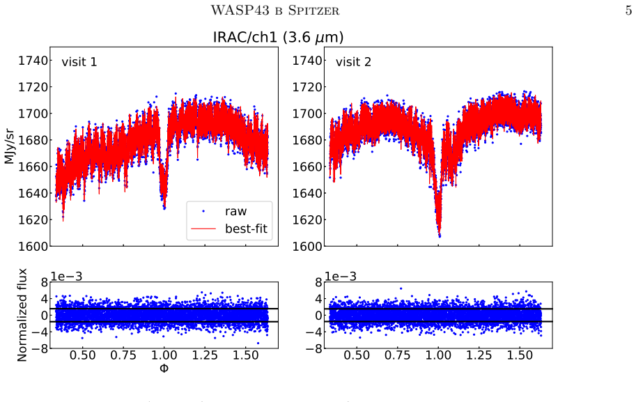
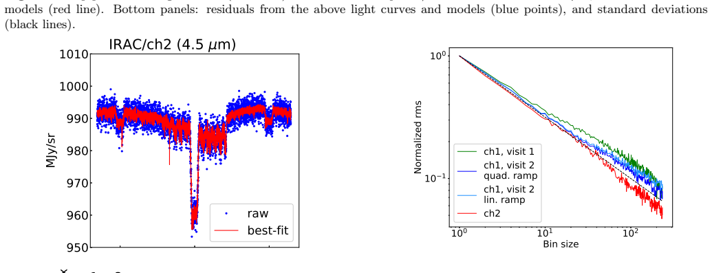
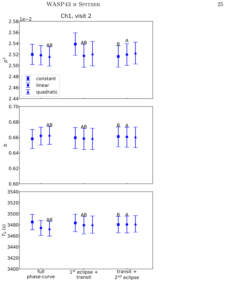
The machinery that carries the argument is wavelet pixel-ICA, a blind source-separation method: it applies a one-level Daubechies-4 discrete wavelet transform to each of the 25 pixel time series in the stellar aperture and then decomposes the set into statistically maximally independent components, so that one component carries the transit/eclipse/phase-curve signal and the others absorb the instrumental systematics without a prescribed functional form. The second, equally decisive piece of machinery is the ramp-model choice for the second 3.6 μm visit: BIC, AIC, CAIC, DIC, and Bayesian evidence all prefer a quadratic ramp, but the authors override that selection because the quadratic solution forces the nightside flux to negative values and its two ramp coefficients correlate with the inferred nightside flux at Pearson coefficient ≈ 0.6, whereas the linear-ramp solution is physically plausible and only weakly correlated (PCC ≈ 0.1). A grid of 2D-ATMO circulation models — with 1×, 3×, and 10× solar metallicity, varying cloud-top pressure, and a fixed 4 km/s substellar zonal wind — then provides the comparison surface on which the re-derived parameters succeed where the original parameters failed.
What would settle it
Take a new 4.5 μm phase curve of WASP43 b and reduce it without committing to a ramp model: if the nightside flux again lands near zero, or the hotspot offset returns to a large eastward shift, the warmer nightside reported here is a detrending artifact. A cheaper check is to apply a Gaussian-process detrending, which marginalizes over ramp shapes, to the archived second 3.6 μm visit and see whether the nightside flux remains positive when the quadratic ramp is not set aside by hand.
Extended reading notes
Core claim
The central claim is that the earlier portrait of WASP43 b as a nearly stagnant atmosphere — almost no nightside emission and a large eastward hotspot — was an artifact of the detector-ramp modeling. When the raw pixel time series are separated into astrophysical signal and instrumental components by wavelet pixel-ICA, the nightside brightness temperature comes out near 1016 K at 3.6 μm in the first visit and near 837 K in the second visit when a linear ramp is adopted, against the 2σ upper limits reported originally, and near 700 K at 4.5 μm; the hotspot offset at 4.5 μm shrinks to 11.3° ± 2.1° east of the substellar point, and the two 3.6 μm visits become consistent within about 1σ. The statistically preferred quadratic ramp for the second 3.6 μm visit is set aside because it drives the nightside flux unphysically negative and its coefficients are strongly correlated with the inferred nightside flux (Pearson coefficient ≈ 0.6), whereas the linear-ramp solution is physically plausible and only weakly correlated. Interpreting the fluxes as blackbody emission gives a circulation efficiency of about 0.1–0.3 instead of the near-zero value claimed by the original study, and a grid of 2D-ATMO circulation models with a high, thin cloud deck (cloud-top pressure near $10^{-3}$–$10^{-2}$ bar) reproduces the measured phase-curve parameters, while cloud-free models are rejected at 4–8σ in nightside flux.
Load-bearing premise
The revision rests on one modeling choice: for the second 3.6 μm observation the paper sets aside the quadratic detector-ramp model that every statistical test prefers, because it drives the nightside flux to unphysical negative values, and adopts the linear ramp instead; if the quadratic ramp is the true detector behavior, the second-visit nightside is consistent with zero and the 3.6 μm nightside temperature claim loses its main pillar.
Editorial extensions
If this is right
- If the reanalysis is right, WASP43 b moves from the canonical example of a non-circulating hot Jupiter to a planet with moderate heat redistribution (ε ≈ 0.1–0.3), in line with the empirical irradiation–efficiency trend established for other planets.
- The 4.5 μm data become consistent with circulation models of near-solar metallicity carrying a high, thin cloud deck (cloud-top pressure ≈ $10^{-3}$ bar), and cloud-free models are excluded at 4–8σ in nightside flux.
- The two 3.6 μm visits being consistent at about 1σ removes the basis for discarding one of them, so future analyses of this planet can use the full data set.
- The retrieved transit parameters are degenerate with the stellar limb-darkening model at the 400–700 ppm level, a systematic floor that will matter for the next generation of space observatories.
- Transit-only analyses of these data are biased by roughly 100 ppm in transit depth because of the flat-baseline assumption, and the provided scaling relation $\Delta p^2 \approx (\sigma/F)\sqrt{N_{\rm tot}/(N_{\rm in}N_{\rm out})}$ lets observers choose baselines that keep this bias below the noise.
Reading between the lines
- A generalizable procedural lesson follows: when a detector-ramp parameter correlates strongly with an astrophysical parameter (the quadratic-ramp coefficients versus nightside flux, PCC ≈ 0.6), information-criterion rankings can select unphysical models; reporting these correlations alongside BIC/AIC would make future reanalyses of phase-curve data much easier to adjudicate.
- If the warmer nightside is real, the apparent differences between visits and between wavelengths become evidence of evolving nightside clouds — a prediction that can be tested directly by a new 4.5 μm observation, which should catch the nightside flux varying between epochs.
- The same blind-separation pipeline could be run on archived phase curves of other hot Jupiters previously classified as low-efficiency; some of those classifications may also be detrending artifacts rather than real atmospheric states.
- The analytic error-scaling relation of the paper, $\Delta p^2 \approx (\sigma/F)\sqrt{N_{\rm tot}/(N_{\rm in}N_{\rm out})}$, can be inverted for scheduling: beyond roughly three transit durations of out-of-transit baseline, extra observing time buys little transit-depth precision, so the marginal time is better spent on eclipse and phase coverage.
Signed reviews
Editorial analysis
A structured set of objections, weighed in public.
Referee Report
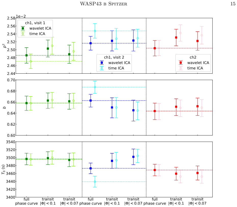
Summary. The paper presents an independent reanalysis of three Spitzer/IRAC phase curves of the hot Jupiter WASP43 b (two visits at 3.6 μm and one at 4.5 μm) using the wavelet pixel-ICA blind source-separation method. The authors report higher nightside temperatures, smaller hotspot offsets, greater consistency between the two 3.6 μm visits, and better agreement with atmospheric circulation models than the original Stevenson et al. (2017) analysis. They also examine the dependence of retrieved transit parameters on stellar limb-darkening models, perform half-phase-curve and transit/eclipse-only analyses, and derive an analytical scaling formula for transit-depth uncertainties as a function of observing duration. The central astrophysical conclusion is that the circulation efficiency of WASP43 b is roughly 0.1–0.3 rather than the near-zero value claimed by S17, which would resolve a long-standing mismatch between observations and circulation models.
Significance. If the main claims hold, the paper resolves a significant discrepancy in the hot-Jupiter literature: the extremely low circulation efficiency inferred by Stevenson et al. (2017) has been difficult to reconcile with 3D atmospheric circulation models, and the present analysis provides a credible alternative measurement that brings WASP43 b into line with empirical irradiation-temperature trends. The paper is methodologically transparent and careful in several important ways: it tests multiple ramp models and two ICA implementations, analyzes half phase curves as a consistency check, inflates weighted-average error bars when individual visits disagree, and explicitly discloses limitations, including the possibility that the true uncertainties on the 3.6 μm peak offsets exceed the nominal error bars. These strengths make the analysis a valuable contribution regardless of the ultimate resolution of the model-selection question.
major comments (3)
- [Section 5.1, Table 6] The central nightside-temperature and inter-visit-consistency claims depend on discarding the BIC/AIC/CAIC/DIC/Bayesian-evidence-preferred quadratic ramp model for the second 3.6 μm visit in favor of a linear ramp model. The justification given is physical plausibility (the quadratic solution yields F_night = (-1.6 ± 1.9) × 10^-4) and the strong correlation between the nightside flux and the quadratic ramp coefficients (PCC ~ 0.6). However, the paper explicitly states in Section 5.2 that the quadratic solution 'cannot [be] rule[d] out as physically impossible,' and it does not perform a Gaussian-process cross-check, which it acknowledges as a possible alternative. Because the positive nightside flux (3.0 ± 1.5) × 10^-4 and the resulting weighted 3.6 μm result in Table 4 are direct consequences of this model-selection decision, the claim that the two 3.6 μm visits are consistent at the ~1σ level is not yet established with the level of confidence claimed. I recommend adding a quantitative test—for example, a Gaussian-process detrending of the second visit, or synthetic-injection experiments showing that a known phase-curve signal is recovered without bias under the linear-ramp assumption—or alternatively presenting the nightside flux as model-dependent and substantially weakening the inter-visit consistency claim.
- [Section 4.1, Table 4] Even if one accepts the linear-ramp model for the second 3.6 μm visit, the reported uncertainties do not account for model-selection uncertainty. The difference between the linear-ramp and quadratic-ramp nightside fluxes is 3.0×10^-4 minus (-1.6×10^-4) = 4.6×10^-4, which is roughly three times the quoted uncertainty on the individual linear-ramp measurement and larger than the 1.26× inflation factor applied to the weighted F_night^MIN in Table 4. The paper should add a systematic error term representing the difference between plausible ramp models (or report the nightside flux as a range spanning both models), because the current Table 4 understates the total uncertainty in the headline 3.6 μm nightside result.
- [Section 5.3, Figures 9-10] The claim that the observations show 'greater similarity with the predictions of the atmospheric circulation models' is overstated relative to the evidence presented. The 3.6 μm dayside flux is higher than all models in the grid by roughly 2–4σ (the paper reports discrepancies of ~150 ppm at 2σ and ~300 ppm at 4σ for solar and 3× solar metallicity), and no single model reproduces both channels within the quoted errors: the best 3.6 μm model has 10× solar metallicity with P_cloud = 2×10^-2 bar, while the best 4.5 μm model has 1× or 3× solar metallicity with P_cloud = 10^-3 bar. The statement that 'a range of models ... can reproduce all of the measured phase curve parameters within less than 2σ' does not support the stronger conclusion of good agreement. The paper should either qualify the atmospheric-model comparison as a loose consistency check or provide a formal statistical comparison (e.g., a joint likelihood over both channels) before claiming that the model grid supports the inferred circulation efficiency.
minor comments (4)
- [Section 4.1] There is a typo: 'unphyisical' should be 'unphysical' in the sentence 'We discarded the (unphyisical) results obtained for the second 3.6 μm visit.'
- [Section 5.4, References] The text cites 'Mendonça et al. (2018b)' but does not distinguish it from the first Mendonça et al. (2018) reference at the point of citation; please introduce both papers explicitly (e.g., M18 vs. Mendonça et al. 2018b) in the text so the reader can connect the citations to the reference list.
- [Appendix A, Equation A5] The statement that the approximation Fin ≈ Fout affects Delta p2 by less than 0.1% for transit depths up to 3% would benefit from a brief derivation or a reference; as written, the reader cannot verify this bound without re-deriving it.
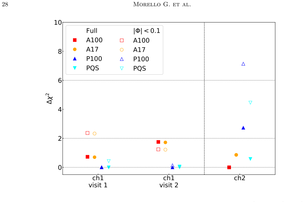
- [Figure 4 and Figures 18-20] The legends and captions use similar color shades (blue and dodger blue) for the quadratic and linear ramp models of the second 3.6 μm visit; adding distinct marker styles (e.g., filled vs. open symbols) would improve accessibility, since the shades are hard to distinguish in printed grayscale.
Circularity Check
No significant circularity: the phase-curve retrieval is a blind, externally benchmarked reduction, and the model-selection and atmospheric-model caveats are transparent limitations rather than circular constructions.
full rationale
The central measurements are obtained by applying the wavelet pixel-ICA method to the raw Spitzer/IRAC time series, with the astrophysical phase-curve parameters determined simultaneously with instrumental ramp parameters. The method is not defined in terms of the target nightside temperatures or hotspot offsets, and the paper's key equations (phase-curve model in Eq. 1 and brightness-temperature inversion in Eq. 2) are standard forward/inversion relations rather than self-referential constructions. The 3.6 um nightside claim is subject to a real model-selection ambiguity: all information criteria prefer the quadratic ramp for visit 2, and the paper adopts the linear ramp on physical-plausibility grounds while explicitly reporting both solutions, including the statement that 'we cannot rule out this solution as physically impossible' (Section 5.2). This is a transparent selection bias and a robustness caveat, not a fitted input renamed as a prediction, and it does not make the retrieval circular by construction. The atmospheric-model comparison (Section 5.3) uses a grid from 2D-ATMO, with metallicity and cloud-top pressure scanned after the fact and a cloud deck added 'in order to reproduce the low fluxes on the nightside'; the resulting agreement is therefore a postdiction rather than a blind prediction, but the measured phase-curve parameters do not depend on those models, and the authors do not claim the models are required to produce the data reductions. The self-citations to Morello et al. (2015, 2016) and Tremblin et al. (2017) are method citations, and the ICA pipeline is independently benchmarked against Ingalls et al. (2016) and compared with other state-of-the-art pipelines; they are not load-bearing unique-force arguments. The paper's stated limitations, such as not pursuing the Gaussian-process cross-check and the correlated-noise caveats, are explicitly acknowledged and do not hide a definitional reduction. Accordingly, no circular step meeting the evidentiary standard can be exhibited.
Assumptions & free parameters
free parameters (6)
- Phase curve harmonic coefficients c0-c4 =
per visit; final values in Table 4
- Instrument ramp coefficients (constant, linear, quadratic) =
per visit; ramp model chosen by BIC plus physical plausibility
- Stellar limb-darkening coefficient set choice =
Table 3: A17, A100, P100, PQS
- Cloud top pressure in 2D-ATMO models =
best matches: 1e-3 bar (4.5 μm), 2e-2 bar (3.6 μm)
- Cloud absorption coefficient =
2.5 m^2 kg^-1
- Atmospheric metallicity grid values =
1x, 3x, 10x solar
assumptions (5)
- standard math The Mandel & Agol (2002) transit model accurately describes the transit and eclipse shapes.
- domain assumption The exoplanet phase curve is described by the harmonic series in Equation (1), with fundamental and first harmonic terms.
- domain assumption ICA separates astrophysical signal from instrument systematics, and the wavelet transform preserves the signal of interest.
- domain assumption Gaussian noise model for the residuals, with error bars inflated by the Interference-to-Signal-Ratio term.
- ad hoc to paper Physical plausibility (non-negative nightside flux) is a valid criterion for selecting the ramp model over BIC preference.
Cite this review
Pith. "Pith review of An independent analysis of the Spitzer/IRAC phase curves of WASP43 b." pith.science (2026). https://pith.science/paper/7MDMUBH3
@misc{pith2026190806741,
  author       = {Pith},
  title        = {Pith review of: An independent analysis of the Spitzer/IRAC phase curves of WASP43 b},
  year         = {2026},
  howpublished = {\url{https://pith.science/paper/7MDMUBH3}},
  note         = {Machine review of arXiv:1908.06741}
}
abstract
We present here a reanalysis of the Spitzer Space Telescope phase curves of the hot Jupiter WASP43 b, using the wavelet pixel-Independent Component Analysis, a blind signal-source separation method. The data analyzed were recorded with the InfraRed Array Camera and consisted of two visits at 3.6 $\mu$m, and one visit at 4.5 $\mu$m, each visit covering one transit and two eclipse events. To test the robustness of our technique we repeated the analysis on smaller portions of the phase curves, and by employing different instrument ramp models. Our reanalysis presents significant updates of the planetary parameters compared to those reported in the original phase curve study of WASP43 b. In particular, we found (1) higher nightside temperatures, (2) smaller hotspot offsets, (3) a greater consistency ($\sim$1 $\sigma$) between the two 3.6~$\mu$m visits, and (4) a greater similarity with the predictions of the atmospheric circulation models. Our parameter results are consistent within 1 $\sigma$ with those reported by a recent reanalysis of the same data sets. For each visit we studied the variation of the retrieved transit parameters as a function of various sets of stellar limb-darkening coefficients, finding significant degeneracy between the limb-darkening models and the analysis output. Furthermore, we performed the analysis of the single transit and eclipse events, and we examined the differences between these results with the ones obtained with the whole phase curve. Finally we provide a formula useful to optimize the trade-off between precision and duration of observations of transiting exoplanets.
Figures

Figures from the paper (24 more)









Forward citations
Cited by 1 Pith paper
-
Phase-dependent chemistry of WASP-43 b revealed with a suite of one-, two-, and three-dimensional models
Horizontal quenching at wind speeds ≳500 m/s, plus carbon-sulfur chemistry, explains the MIRI non-detection of night-side methane on WASP-43 b without requiring high metallicity.
Reference graph
Works this paper leans on
-
[1]
- [1] #1 = = ^ ^ ^ .\!\!^ d .\!\!^ h .\!\!^ m .\!\!^ s .\!\!^ @mss
thebibliography [1] 20pt to REFERENCES 6pt =0pt 10pt plus 3pt =0pt =0pt =1pt plus 1pt =0pt =0pt -12pt =13pt plus 1pt =20pt =13pt plus 1pt \@M =10000 =-1.0em =0pt =0pt 0pt =0pt =1.0em @enumiv\@empty 10000 10000 `\.\@m \@noitemerr \@latex@warning Empty `thebibliography' environment \@ifnextchar \@reference \@latexerr Missing key on reference command Each re...
arXiv 2019
-
[2]
1974, IEEE Transactions on Automatic Control, 19, 716
Akaike, H. 1974, IEEE Transactions on Automatic Control, 19, 716
1974
-
[3]
Bean, J. L., Stevenson, K. B., Batalha, N. M., et al. 2018, , in press
work page 2018
-
[4]
Blecic, J., Harrington, J., Madhusudhan, N., et al. 2014, , 781, 116
work page 2014
- [5]
- [6]
-
[7]
Charbonneau, D., Allen, L. E., Thomas Megeath, S., et al. 2005, 626, 523
work page 2005
- [8]
Show all 66 references
-
[9]
H., & Witte, S
Claret, A., Hauschildt, P. H., & Witte, S. 2012, , 546, A14
2012
-
[10]
H., & Witte, S
Claret, A., Hauschildt, P. H., & Witte, S. 2013, , 552, A16
2013
-
[11]
S., & Showman, A
Cooper, C. S., & Showman, A. P. 2005, , 629, L45
2005
-
[12]
B., Agol, E., & Charbonneau, D
Cowan, N. B., Agol, E., & Charbonneau, D. 2007, , 379, 641
2007
-
[13]
B., & Agol, E
Cowan, N. B., & Agol, E. 2011, , 729, 54
2011
-
[14]
1992, Ten Lectures on Wavelets (Philadephia, PA: Society for Industrial and Applied Mathematics)
Daubechies, I. 1992, Ten Lectures on Wavelets (Philadephia, PA: Society for Industrial and Applied Mathematics)
1992
-
[15]
R., Lewis, N
De Wit, J., Wakeford, H. R., Lewis, N. K., et al. 2018, , 2, 214
2018
-
[16]
R., Gillon, M., et al
De Wit, J., Wakeford, H. R., Gillon, M., et al. 2016, , 537, 69
2016
-
[17]
2015, , 450, 1879
Espinoza, N., & Jord\'an, A. 2015, , 450, 1879
2015
-
[18]
M., Aigrain, S., Gibson, N., et al
Evans, T. M., Aigrain, S., Gibson, N., et al. 2015, , 451, 680
2015
-
[19]
G., Hora, J
Fazio, G. G., Hora, J. :L., Allen, L. E., et al. 2004, , 154, 10
2004
-
[20]
J., Cooper, C
Fortney, J. J., Cooper, C. S., Showman, A. P., Marley, M. S., & Freedman, R. S. 2006, , 652, 746
2006
-
[21]
Gibson, N. P. 2014, , 445, 3401
2014
-
[22]
R., Collier Cameron, A., et al
Hellier, C., Anderson, D. R., Collier Cameron, A., et al. 2011, , 535, L7
2011
-
[23]
Howarth, I. D. 2011, , 418, 1165
2011
-
[24]
2013, , 553, A6
Husser, T.-O., Wende-von Berg, S., Dreizler, S., et al. 2013, , 553, A6
2013
-
[25]
2000, Neural Networks, 13, 411
Hyv\"arinen, A., & Oja, E. 2000, Neural Networks, 13, 411
2000
-
[26]
G., Krick, J
Ingalls, J. G., Krick, J. E., Carey, S. J., et al. 2016, 152, 44
2016
-
[27]
IRAC Instrument & Instrument Support Teams 2015, IRAC Instrument Handbook, v.2.1.2, http://irsa.ipac.caltech.edu/data/SPITZER/docs/irac/iracinstrumenthandbook/
2015
-
[28]
P., Fortney, J
Kataria, T., Showman, A. P., Fortney, J. J., et al. 2015, , 801, 86
2015
-
[29]
& Cowan, N
Keating, D. & Cowan, N. B. 2017, , 849, L5
2017
-
[30]
D., & Showman, A
Komacek, T. D., & Showman, A. P. 2016, , 821, 16
2016
-
[31]
L., D \'e sert, J.-M., et al
Kreidberg, L., Bean, J. L., D \'e sert, J.-M., et al. 2014, , 793, L27
2014
-
[32]
E., Ingalls, J., Carey, S., et al
Krick, J. E., Ingalls, J., Carey, S., et al. 2016, , 824, 27
2016
-
[33]
Kurucz, R. L. 1979, , 40, 1
1979
-
[34]
2002, , 580, L171
Mandel, K., & Agol, E. 2002, , 580, L171
2002
-
[35]
M., Grimm, S
Mendon c a, J. M., Grimm, S. L., Grosheintz, L., & Heng, K. 2016, , 829, 115
2016
-
[36]
M., Malik, M., Demory, B.-O., & Heng, K
Mendon c a, J. M., Malik, M., Demory, B.-O., & Heng, K. 2018, , 155, 150
2018
-
[37]
M., Tsai, S.-M., Malik, M.,Grimm, S
Mendon c a, J. M., Tsai, S.-M., Malik, M.,Grimm, S. L., & Heng, K. 2018, , 869, 107
2018
-
[38]
P., Tinetti, G., et al
Morello, G., Waldmann, I. P., Tinetti, G., et al. 2015, , 802, 117
2015
-
[39]
2015, , 808, 56
Morello, G. 2015, , 808, 56
2015
-
[40]
P., & Tinetti, G
Morello, G., Waldmann, I. P., & Tinetti, G. 2016, , 820, 86
2016
-
[41]
D., & Homeier, D
Morello, G., Tsiaras, A., Howarth, I. D., & Homeier, D. 2017, , 154, 111
2017
-
[42]
R., & Lester, J
Neilson, H. R., & Lester, J. B. 2013, , 554, A98
2013
-
[43]
R., & Lester, J
Neilson, H. R., & Lester, J. B. 2013, , 556, A86
2013
-
[44]
Perez-Becker, D., & Showman, A. P. 2013, , 776, 134
2013
-
[45]
Raftery, A. E. 1995, Sociological Methodology, 25, 111
1995
-
[46]
C., & Cowan, N
Schwartz, J. C., & Cowan, N. B. 2015, , 449, 4192
2015
-
[47]
C., Kashner, Z., Jovmir, D., & Cowan, N
Schwartz, J. C., Kashner, Z., Jovmir, D., & Cowan, N. B. 2017, , 850, 154
2017
-
[48]
1978, The Annals of Statistics, 6, 461
Schwarz, G. 1978, The Annals of Statistics, 6, 461
1978
-
[49]
2003, , 585, 1038
Seager, S., & Mall\'en-Ornelas, G. 2003, , 585, 1038
2003
-
[50]
P., & Guillot, T
Showman, A. P., & Guillot, T. 2002, , 385, 166
2002
-
[51]
J., Best, N
Spiegelhalter, D. J., Best, N. G., Carlin, B. P., & van der Linde, A. 2002, Journal of the Royal Statistical Society Series B, 64, 583
2002
-
[52]
B., Harrington, J., Fortney, J
Stevenson, K. B., Harrington, J., Fortney, J. J., et al. 2012, , 754, 136
2012
-
[53]
B., D\'esert, J.-M., Line, M
Stevenson, K. B., D\'esert, J.-M., Line, M. R., et al. 2014, Science, 346, 838
2014
-
[54]
B., Line, M
Stevenson, K. B., Line, M. R., Bean, J. L., et al. 2017, , 153, 68
2017
-
[55]
Taylor, J. R. 1996, An Introduction to Error Analysis (2nd ed.; University Science Books)
1996
-
[56]
2008, ITNN, 19, 421
Tichavsk\'y, P., Koldovsk\'y, Z., Yeredor, A., G\'omez-Herrero, G., & Doron, E. 2008, ITNN, 19, 421
2008
-
[57]
S., Mourier, P., et al
Tremblin, P., Amundsen, D. S., Mourier, P., et al. 2015, , 804, L17
2015
-
[58]
J., et al
Tremblin, P., Chabrier, G., Mayne, N. J., et al. 2017, , 841, 30
2017
-
[59]
2010, , 7737, 773716
Wu, X., Roby, T., & Ly, L. 2010, , 7737, 773716
2010
-
[60]
T., Lewis, N
Zellem, R. T., Lewis, N. K., Knutson, H. A., et al. 2014, , 790, 53
2014
-
[61]
Zhang, X., & Showman, A. P. 2017, , 836, 73
2017
-
[62]
2012, RSPTA, 370, 2765
Allard, F., Homeier, D., & Freytag, B. 2012, RSPTA, 370, 2765
2012
-
[63]
2008, Biometrika, 95, 759
Chen, J., & Chen, Z. 2008, Biometrika, 95, 759
2008
-
[64]
J., & Quinn, B
Hannan, E. J., & Quinn, B. G. 1979, Journal of the Royal Statistical Society Series B (Methodological), 41, 190
1979
-
[65]
S., Behrenz, L., & Shukur, G., Performances of Model Selection Criteria When Variables are Ill Conditioned, Computational Economics, 2017 (DOI 10.1007/s10614-017-9682-8)
Karlsson, P. S., Behrenz, L., & Shukur, G., Performances of Model Selection Criteria When Variables are Ill Conditioned, Computational Economics, 2017 (DOI 10.1007/s10614-017-9682-8)
2017 doi
-
[66]
1976, Suri-Kagaku (Mathematical Sciences), 153, 12
Takeuchi, K. 1976, Suri-Kagaku (Mathematical Sciences), 153, 12
1976
Reviewed August 14, 2026 · model on record in the stance chip above.
Discussion (0). Continue with ORCID to comment.