REVIEW 3 major objections 4 minor 55 references
Machine Learning Classifiers for Intermediate Redshift Emission Line Galaxies
T0 review · 3 major / 4 minor · reviewed 2026-08-14 · deepseek-v4-flash
Pith's one-line read A random forest trained on low-redshift galaxies can classify intermediate-redshift emission-line galaxies into four excitation classes using only optical data.
desk verdict A solid low-redshift classifier benchmark with public code; the intermediate-redshift application is plausible but not validated, and the accuracy claims should be reframed accordingly. read the letter →
The pith
A machine-rendered reading of the paper's core claim, the machinery that carries it, and where it could break.
The reading
What carries the argument
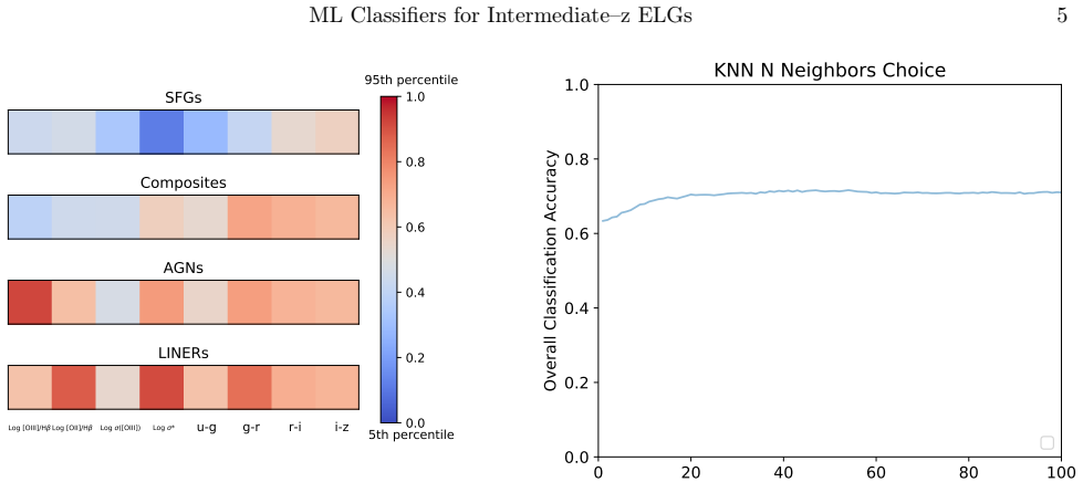
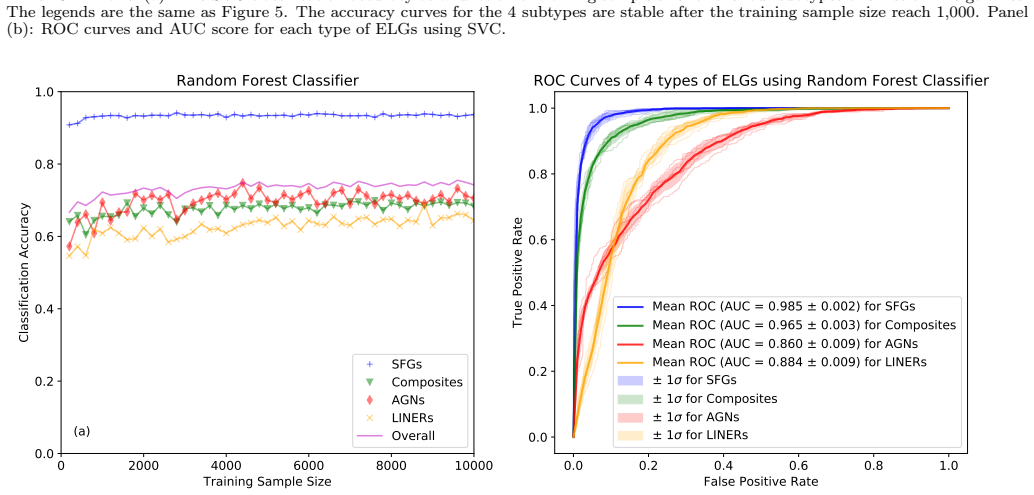
The load-bearing object is a random forest classifier—an ensemble of decision trees whose votes assign each galaxy a class—trained on low-redshift BPT labels with eight features: four spectroscopic ($[\mathrm{O\,III}]/\mathrm{H}\beta$, $[\mathrm{O\,II}]/\mathrm{H}\beta$, $[\mathrm{O\,III}]$ line width, stellar velocity dispersion $\sigma_*$) and four rest-frame colors ($u-g$, $g-r$, $r-i$, $i-z$) k-corrected to $z=0.1$. The random forest was selected after comparing k-nearest neighbors, support vector classifier, and a multi-layer perceptron; it had the highest average area-under-the-ROC-curve score (0.931) and the best balance of per-class accuracies. Feature importance in the trained forest shows that $[\mathrm{O\,III}]/\mathrm{H}\beta$, the $[\mathrm{O\,III}]$ line width, and $g-r$ do most of the work, which is consistent with earlier two-dimensional diagnostics built from the same physics. The same machinery, with only the four spectroscopic features, retains most of the performance, which is what makes the method usable when imaging is absent.
What would settle it
Take a few hundred $0.32<z<0.8$ galaxies with published rest-frame near-infrared spectra covering $[\mathrm{N\,II}]/\mathrm{H}\alpha$ and $[\mathrm{S\,II}]/\mathrm{H}\alpha$, classify them by the standard BPT criteria, and compare with the random forest predictions; if the per-class agreement lies well below the reported 93.4%, 69.4%, 71.8%, and 65.7% accuracies—particularly because composite and LINER predictions drift systematically with redshift—the transfer assumption is falsified.
Extended reading notes
Core claim
The central claim is that a random forest classifier, trained on 28,869 low-redshift ($z<0.32$) galaxies whose labels come from the BPT emission-line diagnostic diagram (the standard $[\mathrm{O\,III}]/\mathrm{H}\beta$ versus $[\mathrm{N\,II}]/\mathrm{H}\alpha$ classification), correctly transfers the four-way classification to 49,272 galaxies at $0.32<z<0.8$. The transfer works because the classifier learns the boundary between classes in a feature space made only of quantities available from optical spectra and broad-band photometry at those redshifts. On a held-out low-redshift test sample the reported accuracies are 93.4% (star-forming), 69.4% (composite), 71.8% (AGN), and 65.7% (LINER), with the four-feature spectroscopic-only version only a few percent lower. The paper's direct evidence for the high-redshift transfer is that the stacked rest-frame 3400–5050 Å spectra of the intermediate-$z$ classes closely match the stacked spectra of the same classes defined by BPT at low $z$, and that the intermediate-$z$ class counts fall where the kinematic–excitation and mass–excitation diagrams would put them. This establishes, conditionally on that consistency, that a four-subtype physical classification of intermediate-redshift galaxies is achievable from optical data alone.
Load-bearing premise
The whole transfer rests on the assumption that the relation between the eight measurable features and the four physically defined classes is the same at $0.32<z<0.8$ as it is at $z<0.32$; at the higher redshifts there is no direct $[\mathrm{N\,II}]/\mathrm{H}\alpha$ or $[\mathrm{S\,II}]/\mathrm{H}\alpha$ ground truth, only stacked-spectrum consistency.
Editorial extensions
If this is right
- Surveys at $0.32<z<0.8$ can obtain four-type classifications for each galaxy in real time from spectra plus photometry, without waiting for near-infrared follow-up; the paper classifies all 49,272 intermediate-redshift galaxies this way.
- A spectra-only random forest retains most of the accuracy (92.3%, 63.7%, 67.3%, 60.8%), so the method survives in fields without multi-band imaging.
- The classifier reproduces BPT classifications at low redshift and its intermediate-redshift outputs line up with the kinematic–excitation and mass–excitation boundaries, so it can serve as a star-forming/AGN selection tool that also preserves the composite and LINER distinction.
- The confusion matrix gives practical error budgets: composites leak into star-forming galaxies at 23.8%, AGNs leak into LINERs at 18.8%, and LINERs leak into composites at 28.4%, so class fractions in a survey sample can be corrected.
Reading between the lines
- The high importance of $[\mathrm{O\,III}]$ line width and $[\mathrm{O\,III}]/\mathrm{H}\beta$ suggests the random forest is effectively relearning the kinematic–excitation diagram, with $g-r$ substituting for stellar mass; a testable prediction is that the learned boundary in the line-width-versus-ratio plane should track that demarcation out to higher redshift.
- Because the labels come from low-redshift BPT classifications, the classifier can only be as good as the assumption that the same line-ratio physics separates the classes at higher redshift; a targeted near-infrared sample of a few hundred $0.32<z<0.8$ galaxies would directly calibrate the transfer, something the paper lists as the ideal test but does not perform.
- The method is survey-agnostic in the sense that the four spectroscopic features can be measured by any optical spectrograph, so retraining on a different instrument's line-flux system is a straightforward extension; the reported accuracies are tied to this particular survey's noise properties and should be re-measured per survey.
- Composite galaxies, the hardest class at 69.4% accuracy, are exactly the transition population between star formation and AGN activity; preserving them as a separate class lets one map where that transition happens across cosmic time, provided the confusion matrix is folded into the analysis.
Signed reviews
Editorial analysis
A structured set of objections, weighed in public.
Referee Report
Summary. The paper trains four supervised machine learning classifiers (KNN, SVC, random forest, MLP) on 28,869 SDSS/eBOSS galaxies at z<0.32, labeled into star-forming, composite, AGN, and LINER types using the BPT diagnostic diagram. Input features are [OIII]/Hb, [OII]/Hb, [OIII] line width, stellar velocity dispersion, and four k-corrected colors. The random forest achieves the best AUC scores and per-subtype accuracies of 93.4%, 69.4%, 71.8%, and 65.7%. The authors apply the trained random forest to 49,272 galaxies at 0.32<z<0.8 and compare stacked spectra with BPT-classified low-redshift stacks, concluding that the intermediate-redshift classifications are correct. The public code and trained models are released.
Significance. If valid, the method would fill a real gap: enabling four-type emission-line galaxy classification from optical spectra alone at 0.3<z<0.8, which is currently prevented by the shift of [NII], Ha, and [SII] out of the optical window. This would be useful for DESI, PFS, and 4MOST. The paper's strengths are the systematic comparison of four algorithms with k-fold cross-validation and error bars, the feature-importance analysis, and the release of code and trained models. The main weakness is that the central intermediate-redshift claim rests on an unvalidated transfer of a low-redshift decision boundary, not on direct measurement.
major comments (3)
- [Section 5, Table 2] The accuracies quoted in the abstract (93.4%, 69.4%, 71.8%, 65.7%) and in Section 4.6 are measured on the z<0.32 test sample described in Section 2.1. That sample is selected with S/N>3 on [NII], Halpha, and [SII], and its labels come from the BPT diagram. These numbers are not measured on the 0.32<z<0.8 sample of Section 2.3, which requires S/N>3 only on [OII], Hb, and [OIII] and has no BPT labels. The only evidence for intermediate-z performance is the stacked-spectrum comparison in Figure 14, which the authors themselves state (Section 5) is affected by the stronger-line selection and by AGN/SFG contamination of the composite and LINER stacks. Therefore the central claim that the RF classifier classifies 0.32<z<0.8 ELGs with the quoted accuracies is not supported by the measurements. The paper should either provide direct validation (e.g., near-IR spectroscopy or a simulated transfer test) or be reframed as a low-redshift classifier with an unvalidated application.
- [Section 4.8, Figure 12] The statement that the RF classifier 'gives as consistent a classification as the BPT diagram' is partly circular: the training labels for all z<0.32 galaxies are defined by the same Kauffmann et al. (2003) and Kewley et al. (2006) demarcation lines used to construct Figure 12. Reproducing those lines on the held-out test set is a sanity check, not an independent validation. The comparison with the KEx diagram in Figure 13 is also expected because two of the eight RF features, [OIII]/Hb and sigma([OIII]), are exactly the axes of that diagram; therefore the consistency does not constitute external confirmation of the intermediate-z classification.
- [Section 5] The application to 0.32<z<0.8 assumes that the mapping between the eight features and the BPT-defined physical class is identical to the mapping at z<0.32, but this assumption is not tested. In particular, [OIII]/Hb, which has the highest feature importance (Figure 8), is sensitive to ionization parameter and may evolve with redshift, potentially shifting high-z star-forming galaxies toward the AGN locus. The paper presents no check of this redshift invariance, such as a comparison to the existing small samples with NIR spectroscopy (e.g., MOSDEF), so the transfer of the decision boundary remains an unsupported extrapolation.
minor comments (4)
- [Section 4.6, Table 1] The text reports average AUC scores of 0.892, 0.895, 0.931, and 0.892 for KNN, SVC, RF, and MLP, but Table 1 lists the MLP average as 0.906; the text value should be corrected.
- [Table 1, Table 2] The column headers in Tables 1 and 2 list LINERs before AGNs, while the text consistently gives the order SFGs, composites, AGNs, LINERs; reorder the columns for consistency.
- [Section 4.8] The sentence 'the accuracies of the RF classification for SFGs are 93.4%, 69.4%, 71.8%' should read 'for SFGs, composites, and AGNs, respectively,' because three values are listed.
- [Section 2.2] The citation 'Baldwin, Philips, & Terlevich 1981' contains a typo: the second author is Phillips, as in the reference list.
Circularity Check
The low-z accuracies are genuine held-out scores, but the intermediate-z validation is partly self-referential: the stacked-spectrum and KEx checks reuse the same features the random forest was trained on.
-
self definitional
[Section 5, Figure 14 and concluding paragraph; abstract statement that the stacked spectra are broadly consistent.]
"The spectral shape of RF-classified sources are highly consistent with BPT-classified low redshift ELGs of the same subtype. The [OIII]/Hβ ratios are consistent with expectations, too. This strongly suggests that the RF classifier is correctly classifying the four subtypes of ELGs."
The RF classifier was trained to reproduce BPT labels from eight input features, of which [OIII]/Hβ is the most important (Figure 8). A stack of galaxies assigned to AGN or LINER by the RF will therefore have elevated [OIII]/Hβ by construction, because that ratio is one of the features the decision trees split on. The claimed consistency of the stacked [OIII]/Hβ with BPT expectations is thus partly a restatement of the training procedure rather than an independent confirmation at 0.32<z<0.8. The paper itself notes that the intermediate-z composite and LINER stacks have significantly higher equivalent widths and are contaminated by AGNs and SFGs (Section 5), so this check is not a clean external test.
-
self citation load bearing
[Section 4.8, text accompanying Figure 13.]
"The RF classification results are quite consistent with the KEx and MEx demarcation lines from Zhang & Hao (2018) and Juneau et al. (2011), respectively."
The KEx diagram is cited to Zhang & Hao (2018), a paper by the same first author as the present work. Its two axes, [OIII]/Hβ and σ([OIII]), are also two of the eight features on which the random forest was trained (Section 3). Agreement with a demarcation line built from the same input features and the same low-redshift BPT class definitions does not provide independent ground truth for the 0.32<z<0.8 transfer; it compares two classifiers that share most of their information. The MEx diagram also uses [OIII]/Hβ as its excitation axis, so the consistency is again partly inherited from a shared input feature.
full rationale
The training-and-test procedure for z<0.32 is not circular: the random forest is trained on BPT-labeled galaxies and evaluated on a held-out low-redshift test set with the same labeling scheme, producing the reported accuracies (93.4% SFG, 69.4% composite, 71.8% AGN, 65.7% LINER). Those accuracies are honest measurements of how well the eight features reproduce BPT classes within the low-redshift sample. The circularity enters only in the transfer to 0.32<z<0.8. The paper explicitly states that direct validation would require near-IR spectra for BPT classification ('The ideal method to test our classifications would be to observe the galaxies with near-IR spectra'), and in lieu of that it relies on stacked-spectrum consistency and agreement with KEx/MEx diagrams. The stacked-spectrum argument is partly self-definitional because [OIII]/Hβ is the most important classifier input, so the same ratio appearing consistent in stacks is expected by construction. The KEx diagram is a self-citation using the same two features, so it is not an independent external standard. The abstract's phrasing also invites the reader to attach the low-redshift test accuracies to the intermediate-redshift problem without the redshift qualifier, although the paper's Section 4 clearly computes those accuracies on the z<0.32 test sample. These issues weaken the intermediate-redshift claim, but they do not collapse the low-redshift derivation, which has genuine independent content; hence a moderate circularity score of 4.
Assumptions & free parameters
free parameters (5)
- KNN number of neighbors k =
54
- Random forest n_estimators =
1000
- MLP hidden layer size =
100 neurons
- MLP learning rate and L2 penalty alpha =
0.001 and 0
- Class-balanced training subsample =
not stated
assumptions (5)
- domain assumption The Kauffmann et al. (2003) and Kewley et al. (2006) BPT demarcation lines correctly separate star-forming, composite, AGN, and LINER galaxies.
- domain assumption The relation between the eight input features and the BPT class is redshift-invariant between z<0.32 and 0.32<z<0.8.
- domain assumption Galaxies with S/N>3 in [OII], H-beta, and [OIII] at intermediate redshift are drawn from the same feature distribution as the low-redshift training sample modulo selection effects.
- domain assumption kcorrect template fitting provides reliable rest-frame colors at z=0.1.
- domain assumption Measurement errors on line ratios, line widths, and velocity dispersions are small enough to ignore after the S/N cuts.
Cite this review
Pith. "Pith review of Machine Learning Classifiers for Intermediate Redshift Emission Line Galaxies." pith.science (2026). https://pith.science/paper/3CTIYDQS
@misc{pith2026190807046,
  author       = {Pith},
  title        = {Pith review of: Machine Learning Classifiers for Intermediate Redshift Emission Line Galaxies},
  year         = {2026},
  howpublished = {\url{https://pith.science/paper/3CTIYDQS}},
  note         = {Machine review of arXiv:1908.07046}
}
abstract
Classification of intermediate redshift ($z$ = 0.3--0.8) emission line galaxies as star-forming galaxies, composite galaxies, active galactic nuclei (AGN), or low-ionization nuclear emission regions (LINERs) using optical spectra alone was impossible because the lines used for standard optical diagnostic diagrams: [NII], H$\alpha$, and [SII] are redshifted out of the observed wavelength range. In this work, we address this problem using four supervised machine learning classification algorithms: $k$-nearest neighbors (KNN), support vector classifier (SVC), random forest (RF), and a multi-layer perceptron (MLP) neural network. For input features, we use properties that can be measured from optical galaxy spectra out to $z < 0.8$---[OIII]/H$\beta$, [OII]/H$\beta$, [OIII] line width, and stellar velocity dispersion---and four colors ($u-g$, $g-r$, $r-i$, and $i-z$) corrected to $z=0.1$. The labels for the low redshift emission line galaxy training set are determined using standard optical diagnostic diagrams. RF has the best area under curve (AUC) score for classifying all four galaxy types, meaning highest distinguishing power. Both the AUC scores and accuracies of the other algorithms are ordered as MLP$>$SVC$>$KNN. The classification accuracies with all eight features (and the four spectroscopically-determined features only) are 93.4% (92.3%) for star-forming galaxies, 69.4% (63.7%) for composite galaxies, 71.8% (67.3%) for AGNs, and 65.7% (60.8%) for LINERs. The stacked spectrum of galaxies of the same type as determined by optical diagnostic diagrams at low redshift and RF at intermediate redshift are broadly consistent. Our publicly available code (https://github.com/zkdtc/MLC_ELGs) and trained models will be instrumental for classifying emission line galaxies in upcoming wide-field spectroscopic surveys.
Figures


Figures from the paper (10 more)




Reference graph
Works this paper leans on
-
[1]
Acquaviva, V.\ 2019, arXiv e-prints, arXiv:1901.05978
work page Pith review arXiv 2019
-
[2]
S., Ahumada, R., Almeida, A., et al.\ 2019, , 240, 23
Aguado, D. S., Ahumada, R., Almeida, A., et al.\ 2019, , 240, 23
work page 2019
-
[3]
L., Aird, J., et al.\ 2017, , 835, 27
Azadi, M., Coil, A. L., Aird, J., et al.\ 2017, , 835, 27
work page 2017
-
[4]
A., Phillips, M
Baldwin, J. A., Phillips, M. M., & Terlevich, R.\ 1981, , 93, 5
1981
- [5]
-
[6]
R., Bershady, M
Blanton, M. R., Bershady, M. A., Abolfathi, B., et al.\ 2017, , 154, 28
2017
-
[7]
Boyle, B. J., Shanks, T., Croom, S. M., et al.\ 2000, , 317, 1014
work page 2000
-
[8]
Bradley 1997, Pattern Recognition Volume 30, Issue 7, July 1997, Pages 1145-1159
work page 1997
Show all 55 references
-
[9]
A., et al.\ 2012, , 421, 314
Chen, Y.-M., Kauffmann, G., Tremonti, C. A., et al.\ 2012, , 421, 314
2012
-
[10]
Comparat, J., Zhu, G., Gonzalez-Perez, V., et al.\ 2016, , 461, 1076
2016
-
[11]
S., Bellido-Tirado, O., Chiappini, C., et al.\ 2012, , 8446, 84460T
de Jong, R. S., Bellido-Tirado, O., Chiappini, C., et al.\ 2012, , 8446, 84460T
2012
-
[12]
de la Calleja, J., & Fuentes, O.\ 2004, , 349, 87
2004
-
[13]
J., Lang, D., et al.\ 2019, , 157, 168
Dey, A., Schlegel, D. J., Lang, D., et al.\ 2019, , 157, 168
2019
-
[14]
S., Kneib, J.-P., Percival, W
Dawson, K. S., Kneib, J.-P., Percival, W. J., et al.\ 2016, , 151, 44
2016
-
[15]
W., & Dambre, J.\ 2015, , 450, 1441
Dieleman, S., Willett, K. W., & Dambre, J.\ 2015, , 450, 1441
2015
-
[16]
Fawcett, Pattern Recognition Letters Volume 27, Issue 8, June 2006, Pages 861-874
2006
-
[17]
Ferri, C., Hern \'a ndez-Orallo, J., Modroiu, R., Pattern Recognition Letters 30 (2009) 27?38
2009
-
[18]
& Till, R.J
Hand, D.J. & Till, R.J. Machine Learning (2001) 45: 171. https://doi.org/10.1023/A:1010920819831
2001 doi
-
[19]
E., Sun, Y., et al.\ 2018, , 473, 1108
Hocking, A., Geach, J. E., Sun, Y., et al.\ 2018, , 473, 1108
2018
-
[20]
Huang, X., Domingo, M., Pilon, A., et al.\ 2019, arXiv e-prints, arXiv:1906.00970
2019 arXiv
-
[21]
Jacobs, C., Glazebrook, K., Collett, T., et al.\ 2017, , 471, 167
2017
-
[22]
Jacobs, C., Collett, T., Glazebrook, K., et al.\ 2019, , 484, 5330
2019
-
[23]
Jacobs, C., Collett, T., Glazebrook, K., et al.\ 2019, arXiv e-prints, arXiv:1905.10522
2019 arXiv
-
[24]
M., & Salim, S.\ 2011, , 736, 104
Juneau, S., Dickinson, M., Alexander, D. M., & Salim, S.\ 2011, , 736, 104
2011
-
[25]
M., Tremonti, C., et al.\ 2003, , 346, 1055
Kauffmann, G., Heckman, T. M., Tremonti, C., et al.\ 2003, , 346, 1055
2003
-
[26]
J., Groves, B., Kauffmann, G., & Heckman, T.\ 2006, , 372, 961
Kewley, L. J., Groves, B., Kauffmann, G., & Heckman, T.\ 2006, , 372, 961
2006
-
[27]
J., Dopita, M
Kewley, L. J., Dopita, M. A., Leitherer, C., et al.\ 2013, , 774, 100
2013
-
[28]
J., Maier, C., Yabe, K., et al.\ 2013, , 774, L10
Kewley, L. J., Maier, C., Yabe, K., et al.\ 2013, , 774, L10
2013
-
[29]
Kingma, Diederik P., Ba, Jimmy 3rd International Conference for Learning Representations, San Diego, 2015 arXiv:1412.6980
2015 arXiv
-
[30]
E., Reddy, N
Kriek, M., Shapley, A. E., Reddy, N. A., et al.\ 2015, , 218, 15
2015
-
[31]
Lamareille, F.\ 2010, , 509, A53
2010
-
[32]
Levi, M., Bebek, C., Beers, T., et al.\ 2013, arXiv:1308.0847
2013 arXiv
-
[33]
Lintott, C., Schawinski, K., Bamford, S., et al.\ 2011, , 410, 166
2011
-
[34]
Maraston, C., & Str \"o mb \"a ck, G.\ 2011, , 418, 2785
2011
-
[35]
Marocco, J., Hache, E., & Lamareille, F.\ 2011, , 531, A71
2011
-
[36]
B., Croft, R
Metcalf, R. B., Croft, R. A. C., & Romeo, A.\ 2018, , 477, 2841
2018
-
[37]
1978 Oct;8(4):283-98
Metz, Seminars in Nuclear Medicine. 1978 Oct;8(4):283-98
1978
-
[38]
1999 Jan-Mar;19(1):78-89
Mossman, Medical Decision Making. 1999 Jan-Mar;19(1):78-89
1999
-
[39]
Pedregosa, F., Varoquaux, G., Gramfort, A. et al. JMLR 12, pp. 2825-2830, 2011
2011
-
[40]
E., Tortora, C., Chatterjee, S., et al.\ 2017, , 472, 1129
Petrillo, C. E., Tortora, C., Chatterjee, S., et al.\ 2017, , 472, 1129
2017
-
[41]
Pourrahmani, M., Nayyeri, H., & Cooray, A.\ 2018, , 856, 68
2018
-
[42]
S., Terlevich, E., & Terlevich, R
Rola, C. S., Terlevich, E., & Terlevich, R. J.\ 1997, , 289, 419
1997
-
[43]
L., Shapley, A
Sanders, R. L., Shapley, A. E., Kriek, M., et al.\ 2016, , 816, 23
2016
-
[44]
V.\ 2006, , 371, 972
Stasi \'n ska, G., Cid Fernandes, R., Mateus, A., Sodr \'e , L., & Asari, N. V.\ 2006, , 371, 972
2006
-
[45]
Srinivasan, A., Note on the Locations of Optimal Classifiers in N-Dimensional ROC Space
-
[46]
S., Chiba, M., et al.\ 2014, , 66, R1
Takada, M., Ellis, R. S., Chiba, M., et al.\ 2014, , 66, R1
2014
-
[47]
Tamura, N., Takato, N., Shimono, A., et al.\ 2016, , 9908, 99081M
2016
-
[48]
Tresse, L., Rola, C., Hammer, F., et al.\ 1996, , 281, 847
1996
-
[49]
J., & Tremonti, C.\ 2011, , 742, 46
Trouille, L., Barger, A. J., & Tremonti, C.\ 2011, , 742, 46
2011
-
[50]
R., Konidaris, N
Trump, J. R., Konidaris, N. P., Barro, G., et al.\ 2013, , 763, L6
2013
-
[51]
E.\ 1987, , 63, 295
Veilleux, S., & Osterbrock, D. E.\ 1987, , 63, 295
1987
-
[52]
J., Willmer, C
Weiner, B. J., Willmer, C. N. A., Faber, S. M., et al.\ 2006, , 653, 1027
2006
-
[53]
C., Newman, J
Yan, R., Ho, L. C., Newman, J. A., et al.\ 2011, , 728, 38
2011
-
[54]
G., Adelman, J., Anderson, J
York, D. G., Adelman, J., Anderson, J. E., Jr., et al.\ 2000, , 120, 1579
2000
-
[55]
Zhang, K., & Hao, L.\ 2018, , 856, 171
2018
Reviewed August 14, 2026 · model on record in the stance chip above.
Discussion (0). Continue with ORCID to comment.