REVIEW 4 major objections 5 minor 16 references
Enabling a new detection channel for beyond standard model physics with in-situ measurements of ice luminescence
T0 review · 4 major / 5 minor · reviewed 2026-08-14 · deepseek-v4-flash
Pith's one-line read This paper reports the first in-situ measurement of luminescence yield and decay kinetics in the glacial ice of a neutrino telescope, yielding 5–25 photons per MeV and four decay times, and argues this opens a detection channel for slow…
desk verdict First in-situ ice luminescence measurement in a neutrino telescope medium—genuinely new, but the yield–distance degeneracy needs to be shown before the sensitivity projection is trusted. read the letter →
The pith
A machine-rendered reading of the paper's core claim, the machinery that carries it, and where it could break.
The reading
What carries the argument
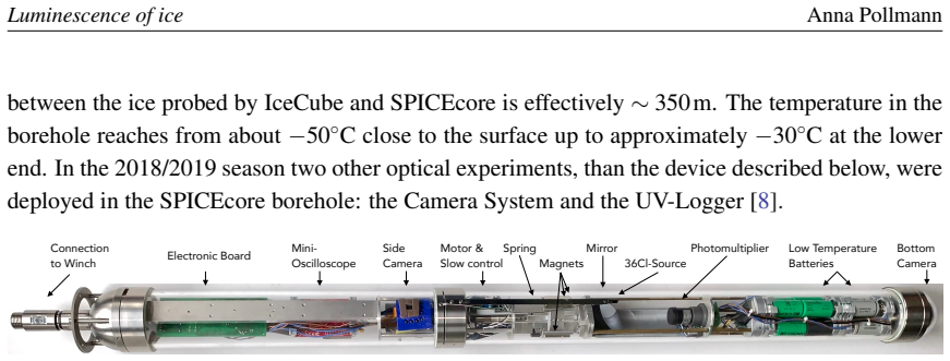
The carrying object is the Luminescence Logger: a quartz-glass pressure vessel housing a chlorine-36 beta source on a spring that can be pushed against the borehole wall, a parabolic mirror that directs emitted photons to a photomultiplier, and an onboard oscilloscope recording timestamps and 120 ns waveforms. The argument runs through a custom ray-tracing simulation in which simulated electron tracks from the source generate Cherenkov and luminescence photons in both the borehole fluid and the ice; the simulation then varies the ice luminescence yield and the average source-to-ice distance to fit the measured trigger rates. The decay kinetics come from the distribution of time intervals between random reference pulses and subsequent detected pulses, which is fit by four exponentials.
What would settle it
A repeat measurement that holds the source-to-ice distance fixed at a value measured independently, for example from the logger's camera images, while fitting the yield would settle whether the reported 5–25 photons per MeV range survives removal of that fit degeneracy; a laboratory bench calibration with a known source-to-ice gap and independently characterized ice optical attenuation would do the same.
Extended reading notes
Core claim
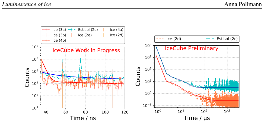
The central claim is that luminescence in South Pole glacial ice is strong enough and slow enough to be seen by a neutrino telescope's optical sensors: after excitation by beta electrons, the ice emits of order 5–25 photons per MeV of deposited energy, with decay components at (2.44 ± 0.21) ns, (189.6 ± 29.9) ns, (5.03 ± 0.06) µs, and (56.10 ± 6.26) µs. Because the emission persists long after the exciting particle has passed, the light is separable from prompt Cherenkov light and from dark noise over a few hundred microseconds. The paper further argues that charged Q-balls and slow magnetic monopoles, which are not relativistic enough to emit Cherenkov light, deposit large energy losses and therefore produce detectable luminescence, making this a new search channel for the observatory.
Load-bearing premise
The photon counts are trustworthy only if the average distance between the radioactive source and the ice wall is known well enough that varying it during the fit cannot compensate for a wrong luminescence yield.
Editorial extensions
If this is right
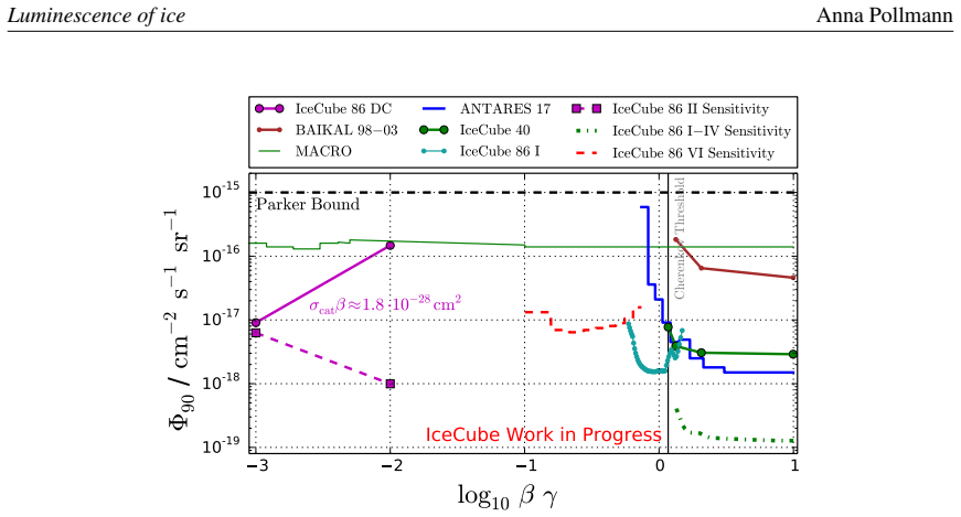
- Existing South Pole optical modules can be used to search for slow magnetic monopoles below about 0.5 c, where they emit no Cherenkov light; the paper reports the first such search reaches a sensitivity roughly an order of magnitude beyond previous limits.
- Charged Q-balls, which emit no Cherenkov light, become detectable through luminescence, with reported yields implying light outputs comparable to monopole nucleon-decay signatures in the parameter ranges shown.
- The four measured decay times give the new channel a timing signature: events whose light lingers on microsecond timescales can be distinguished from prompt muon background.
- Because the measurement was made in glacial ice at temperatures and depths overlapping the detector's fiducial volume, the yield values can be used directly in simulations of new-particle signatures.
- A planned repeat deployment at more depths, with smaller uncertainties and a rough spectral measurement, would identify the specific electronic transitions responsible and map any temperature or impurity dependence.
Reading between the lines
- If the 56 µs decay component is confirmed, a delayed-coincidence trigger requiring a second pulse within tens of microseconds of a first would reject most Cherenkov and photomultiplier noise, sharpening the luminescence channel without new hardware.
- The same measurement protocol could be transplanted to any ice- or water-based detector; the key systematic source-to-wall distance could be calibrated with the logger's own camera images, making the yield extraction more robust.
- The yield's temperature dependence between about -48 °C and -36 °C is not resolved by the three depths tested; if the planned spectrum shows impurity-dominated emission, the yield may vary across the detector as impurities do, and a single measured range would need a depth map before being used to set limits.
Signed reviews
Editorial analysis
A structured set of objections, weighed in public.
Referee Report
Summary. The paper reports a down-hole luminescence logger deployed in the SPICEcore borehole at the South Pole, exposing glacial ice to a Cl-36 beta source and recording single-photon pulses with a photomultiplier. A custom ray-tracing simulation converts measured rates into an ice luminescence yield, reported as roughly 5-25 photons per MeV, and time-difference spectra are fit with four exponential decay components. The results are then applied to estimate the sensitivity of IceCube to slow magnetic monopoles and charged Q-balls, and the work is presented as opening a new luminescence-based detection channel for beyond-standard-model particles.
Significance. If the measurement is robust, it is a first-of-its-kind in-situ determination of luminescence yield and decay kinetics in the actual optical medium of a neutrino telescope, and it directly enables a monopole search that would otherwise be blind below roughly 0.5c. The paper is appropriately preliminary in many places and propagates several relevant instrumental systematic uncertainties, which are real strengths. However, the scientific payoff is conditional on a well-characterized yield extraction and a convincing decay-time fit, because the quoted yield range enters the sensitivity projection nearly linearly.
major comments (4)
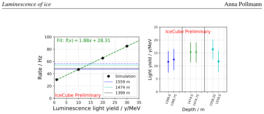
- [Section 3, Figure 4] The yield estimate is obtained by varying both the ice luminescence yield and the average source-to-ice distance, but the paper shows only a resulting one-dimensional yield range and no joint fit surface, prior, or covariance. Because the simulated rate depends on both parameters, the quoted 5-25 photons/MeV is underconstrained unless the distance is marginalized with a physical prior based on the borehole diameter (126.8 mm) and logger geometry. Please show the two-dimensional chi-square or likelihood, the allowed distance range, and the sensitivity of the yield range to the distance prior; without this, the quoted systematic uncertainty cannot be traced, and the degeneracy propagates directly into the monopole sensitivity projection in Section 4 and Figure 7.
- [Section 3, systematic uncertainties] The list of propagated uncertainties (mirror reflectivity, PMT quantum efficiency, source emission rate, scattering and absorption lengths) omits several inputs that enter the rate-to-yield conversion shown in Figure 4, namely the fixed 6 mV offline threshold, the approximately 800 ns deadtime, the stated 95.5% oscilloscope trigger accuracy, and the assumption that Estisol luminescence and dark noise are approximately constant backgrounds. Each of these should either be assigned a numerical uncertainty or be explicitly justified as negligible, since the linear calibration f(x)=1.88x+28.31 in Figure 4 means any rate-scale error shifts the yield directly.
- [Section 3, decay-time fit] The four decay constants (2.44 ns, 189.6 ns, 5.03 microseconds, 56.10 microseconds) are a central result, but the fit description is too sparse to support them: no fit ranges for amplitudes, no chi-square per degree of freedom or residuals, no discussion of parameter correlations, and no explicit treatment of the 120-800 ns deadtime gap or electronic ringing beyond a dark-noise shape correction. Because Section 5 claims a first measurement of decay kinetics in the detection medium, this fit needs validation, including a comparison with models using different numbers of exponentials and a description of how the random-reference-pulse method is corrected for the trigger rate.
- [Section 4, Figure 7] The monopole sensitivity projection is a headline application, yet it is drawn as a single dashed line with no band representing the 5-25 photons/MeV yield range. Please state which yield value was used and show how the sensitivity changes across the allowed yield range. Without this, the statement that the luminescence-based search exceeds previous exclusion limits by an order of magnitude is not connected to the measurement uncertainty established in Section 3.
minor comments (5)
- [Throughout] The text contains several typographical and encoding artifacts, including 'chanel' in the Figure 7 caption, 'accurancy', 'IceCubeâ ˘A ´Zs', and '1km 3', which should be corrected before publication.
- [Figure 4] The right panel axis label 'Light yield / /MeV' should be 'photons/MeV', and the numerical yield range should be stated explicitly in the text rather than only visible in the figure.
- [Figure 5] The right panel axis is labeled 'Time / s' while the text says the distribution extends up to 2 ms; the axis unit and the text should be harmonized.
- [Figure 1] The caption sentence containing 'd by different kind of radiations' is garbled, and the legend entries could be clarified to distinguish 'IceCube 2019' from 'IceCube Preliminary'.
- [Section 2] The antifreeze liquid Estisol is introduced without defining its composition or explaining why its luminescence and Cherenkov contributions can be treated as an approximately constant background; a one-sentence justification or reference would help.
Circularity Check
No significant circularity: the measured yield and decay times are extracted from data and then used as forward inputs, not recycled as predictions.
full rationale
The derivation chain is a measurement: the luminescence yield and decay constants are parameters extracted by fitting a ray-tracing simulation to logged rates, not quantities assumed beforehand. Section 3 states: 'The light yield of ice luminescence is varied in the simulation as well as the average distance of the source to the ice. The predicted rates are compared with the measured rates which gives a range of possible values for the luminescence yield of ice per measurement.' This is an inverse problem with the yield as a fitted output. The decay kinetics are likewise obtained from measured pulse-time distributions by a chi-square fit, and the paper explicitly says 'There are no previous measurements to which these values can be compared,' so no imported ansatz fixes the result. Section 4 uses the measured efficiency as an input: the monopole light yield is 'obtained by convoluting the energy loss with the luminescence efficiency obtained above,' and the resulting sensitivity is a forward application, not a self-referential prediction. The only self-citation, Ref. [2], is used to motivate the expectation that highly ionizing particles produce detectable luminescence; it is not used to set the fitted yield or decay times and is therefore not load-bearing. The yield-distance covariance noted by a skeptic is a systematic uncertainty in the fit, not a circular step: the paper does not equate the derived yield with an input or define the yield in terms of the measured monopole sensitivity. I find no step where a claimed prediction reduces by construction to its inputs.
Assumptions & free parameters
free parameters (3)
- Average source-to-ice distance =
not quoted; varied in simulation
- Offline discrimination threshold =
6 mV
- Decay time constants =
2.44 ns, 189.6 ns, 5.03 us, 56.10 us
assumptions (5)
- domain assumption Electrons from the 36Cl source deposit energy in ice and Estisol as simulated in Ref [9].
- domain assumption Photons are emitted either at the Cherenkov angle or isotropically for luminescence, and propagate with exponential attenuation using SPICEcore attenuation and scattering lengths.
- domain assumption Background rates (dark noise and Estisol emission) are approximately constant, and Estisol luminescence is negligible.
- domain assumption A quenching ratio of electrons to alphas of about 10 applies.
- domain assumption Single-photon pulse timing after a random reference pulse reproduces the decay kinetics.
Cite this review
Pith. "Pith review of Enabling a new detection channel for beyond standard model physics with in-situ measurements of ice luminescence." pith.science (2026). https://pith.science/paper/C4T66HR2
@misc{pith2026190807231,
  author       = {Pith},
  title        = {Pith review of: Enabling a new detection channel for beyond standard model physics with in-situ measurements of ice luminescence},
  year         = {2026},
  howpublished = {\url{https://pith.science/paper/C4T66HR2}},
  note         = {Machine review of arXiv:1908.07231}
}
abstract
The IceCube neutrino observatory uses $1\,\mathrm{km}^{3}$ of the natural Antarctic ice near the geographic South Pole as optical detection medium. When charged particles, such as particles produced in neutrino interactions, pass through the ice with relativistic speed, Cherenkov light is emitted. This is detected by IceCube's optical modules and from all these signals a particle signature is reconstructed. A new kind of signature can be detected using light emission from luminescence. This detection channel enables searches for exotic particles (states) which do not emit Cherenkov light and currently cannot be probed by neutrino detectors. Luminescence light is induced by highly ionizing particles passing through matter due to excitation of surrounding atoms. This process is highly dependent on the ice structure, impurities, pressure and temperature which demands an in-situ measurement of the detector medium. For the measurements at IceCube, a $1.7\,\mathrm{km}$ deep hole was used which {vertically} overlaps with the glacial ice layers found in the IceCube volume over a range of $350\,\mathrm{m}$. The experiment as well as the measurement results are presented. The impact {of the results, which enable new kind of} searches for new physics with neutrino telescopes, are discussed.
Figures


Figures from the paper (4 more)

Reference graph
Works this paper leans on
-
[1]
T. I. Quickenden, S. M. Trotman, and D. F. Sangster, J. Chem. Phys. 77 (1982) 3790
work page 1982
-
[2]
Pollmann in EPJ Web Conf., vol
A. Pollmann in EPJ Web Conf., vol. 164, p. 07019, 2017
work page 2017
-
[3]
M. Duquesne and I. Kaplan, Phys. Radium 21 (1960) 708. (in French); M. D. Tarasov et al., Instrum. Exp. Tech. 50 (2007), no. 6 761–763; H. B. Steen, O. I. Sorensen, and J. A. Holteng, Int. J. Radiat. Phys. Chem. 4 (1972) 75â ˘A¸ S86;Baikal Collaboration, V . Aynutdinov et al.,Astropart. Phys. 29 (2008) 366 â ˘A¸ S 372. Original description in I. I. Trofime...
work page 1960
- [4]
-
[5]
IceCube Collaboration, PoS(ICRC2017)1060 (2018)
work page 2018
-
[6]
IceCube Collaboration, M. G. Aartsen et al., JINST 12 (2017) P03012
2017
-
[7]
SPICEcore Collaboration, Annals of Glaciology 55 (2014) 137–146
work page 2014
-
[8]
IceCube Collaboration, PoS (ICRC2019) 847 (these proceedings)
IceCube Collaboration, PoS(ICRC2019)926 (these proceedings). IceCube Collaboration, PoS (ICRC2019) 847 (these proceedings)
Show all 16 references
-
[9]
Allision et al., Nucl
SPICEcore Collaboration, J. Allision et al., Nucl. Instrum. Methods Phys. Res. 835 (2016) 186–225
2016
-
[10]
Kusenko, Phys.Lett.B 405 (1997) 108
A. Kusenko, Phys.Lett.B 405 (1997) 108
1997
-
[11]
Kusenko et al., Phys.Rev.Lett
A. Kusenko et al., Phys.Rev.Lett. 80 (1998) 3185–3188
1998
-
[12]
Rubakov,Rep
V . Rubakov,Rep. Prog. Phys. 51 (1988) v
1988
-
[13]
Lauber, EPJ Web Conf
F. Lauber, EPJ Web Conf. 182 (2017) 02071
2017
-
[14]
Chen et al
T. Chen et al. in 22nd ACM SIGKDD International Conference on Knowledge Discovery and Data Mining, p. 785â ˘A¸ S794, 2016
2016
-
[15]
IceCube Collaboration, PoS(ICRC2015)1211 (2016)
2016
-
[16]
IceCube Collaboration, M. G. Aartsen and et.al, Eur . Phys. J.C74 (July, 2014). 2938; IceCube Collaboration, M. G. Aartsen and et.al, Eur . Phys. J.C76 (2016) 1 â ˘A¸ S 16;Baikal Collaboration, V . Aynutdinov et al., Astropart. Phys. 29 (2008) 366 â ˘A¸ S 372;MACRO Collaborati...
2016
Reviewed August 14, 2026 · model on record in the stance chip above.
Discussion (0). Continue with ORCID to comment.