Herschel map of Saturn's stratospheric water, delivered by the plumes of Enceladus

C. Jarchow; E. Lellouch; F. Billebaud; G.S. Orton; H. Feuchtgruber; L.N. Fletcher; L. Rezac; M. Dobrijevic; M. Rengel; P. Hartogh

REVIEW 3 major objections 4 minor 120 references

Herschel map of Saturn's stratospheric water, delivered by the plumes of Enceladus

T0 review · 3 major / 4 minor · reviewed 2026-08-14 · deepseek-v4-flash

Challenge this review Re-run · record.json Download PDF Read on arXiv ↗ Review JSON

Pith's one-line read Saturn's stratospheric water is concentrated in an equatorial band, pointing to Enceladus's plumes as its main source.

desk verdict First disk-resolved H2O map robustly kills the uniform-IDP picture, but the Enceladus attribution is more interpretive than the abstract lets on. read the letter →

arxiv 1908.07399 v1 pith:XDBUAVPB submitted 2019-08-20 astro-ph.EP

T. Cavalié , V. Hue , P. Hartogh , R. Moreno , E. Lellouch , H. Feuchtgruber , C. Jarchow , T. Cassidy

show 8 more authors

L.N. Fletcher F. Billebaud M. Dobrijevic L. Rezac G.S. Orton M. Rengel T. Fouchet S. Guerlet

This is my paper · ORCID

classification astro-ph.EP

keywords SaturnstratospherestratosphericwaterEnceladusplumesHerschelPACSmeridionaldistributionneutraltorusradiativetransferringinfall

verification ladder T0 review T1 audit T2 compute T3 formal

The pith

A machine-rendered reading of the paper's core claim, the machinery that carries it, and where it could break.

The reading

Since water was first detected in the stratospheres of the giant planets, its origin has been an open question: it could fall in from interplanetary dust, from icy rings or moons, or from comet impacts. This paper uses the first disk-resolved far-infrared map of Saturn's stratospheric water, taken by the PACS instrument on a space observatory, to separate those possibilities. It argues that the water is not spread evenly with latitude but is concentrated in a band centered on Saturn's equator, with a peak mole fraction of 1.1 ppb and a half-width of 25 degrees. That shape matches the predicted fall-in from the neutral water torus fed by Enceladus's plumes, and the data reject a uniform, dust-like background as the main source. The paper concludes that Enceladus is the main supplier of Saturn's stratospheric water, settling a twenty-year debate with a spatial map rather than a disk-averaged spectrum.

What carries the argument

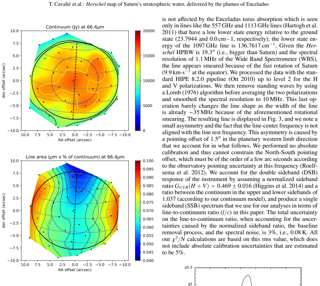
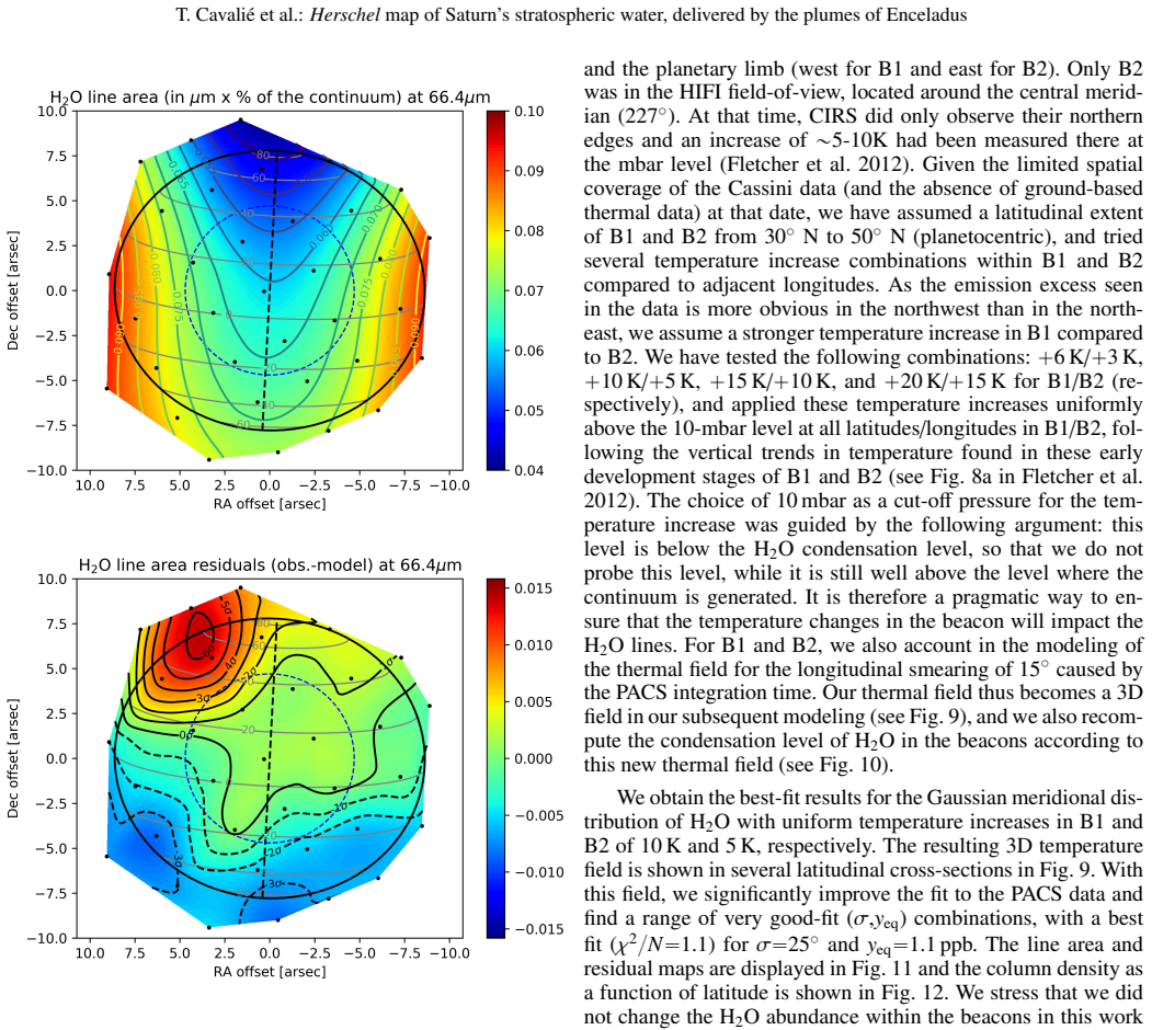
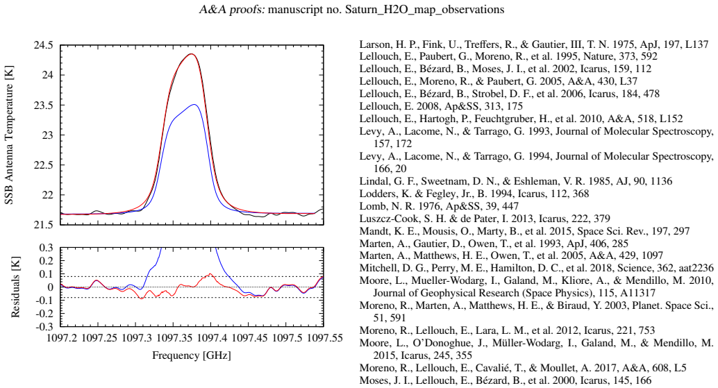
The load-bearing object is the disk-resolved line-area map of the 66.44-micrometer water transition, interpreted with a line-by-line radiative-transfer calculation on a densely sampled three-dimensional grid. The tested water distributions take the form $y_{\mathrm{H_2O}}(\phi)=y_{\mathrm{eq}}\exp(-\phi^2/2\sigma^2)$ above the local condensation level, where $\phi$ is planetocentric latitude, $y_{\mathrm{eq}}$ the equatorial mole fraction, and $\sigma$ the Gaussian half-width; a meridionally uniform profile is the competing interplanetary-dust model. The argument works by convolving synthetic line maps with the instrument beam and comparing them with the 225 observed spectra, first with a storm-free thermal field and then with a three-dimensional field that inserts +10 K and +5 K patches over the two Great Storm beacons so the equatorial excess can be isolated. The same setup produces the disk-averaged 1097 GHz HIFI line, which probes slightly higher altitudes and exposes the residual vertical-profile incompatibility.

What would settle it

Recompute the fits using beacon temperature profiles retrieved directly from contemporaneous Composite Infrared Spectrometer data instead of the four tested uniform increments; if the best-fit Gaussian moves away from $y_{\mathrm{eq}}=1.1$ ppb and $\sigma=25^\circ$, or if a uniform profile becomes acceptable, the central claim is undermined. An independent check is a water map taken at a time without storm beacons, which should show the same equatorial Gaussian without inserted temperature patches.

Watch

Extended reading notes

Core claim

The paper's central claim is that Enceladus, through its plume-fed neutral torus, is the main source of Saturn's stratospheric water. The evidence is the 66.44-micrometer water line map: with the two warm storm beacons added to the thermal field, the observed map is best reproduced by a Gaussian meridional abundance profile centered on the equator, with equatorial mole fraction 1.1 ppb and half-width at half-maximum 25 degrees, giving a normalized chi-squared of 1.1. A meridionally uniform profile, representing interplanetary dust, fails with a normalized chi-squared of 16.2, and a uniform background component is limited to about 0.06 ppb at the 2-sigma level. The water falling from the rings that spacecraft instruments measured in 2017 cannot explain the 2010-2011 observations because that infall appeared later. The paper also reports that adding a vertical gradient above the condensation level reduces, but does not fully remove, the factor-of-five abundance gap between the disk-averaged HIFI line and the disk-resolved PACS map.

Load-bearing premise

The result depends on the assumed temperature and size of the two warm storm vortices: if their actual temperatures, vertical structure, or latitude range differ from the +10 K and +5 K patches used here, the fitted equatorial abundance and width would shift.

Editorial extensions

If this is right

Enceladus's plume-fed neutral torus, not interplanetary dust or the rings, supplied the stratospheric water seen in 2010-2011.
A meridionally uniform dust-like contribution is at most about an order of magnitude fainter than the equatorial source, around 0.06 ppb.
The ring-infall water measured in 2017 cannot be the source of the Herschel-era water; it must have intensified after 2010-2011.
If the input flux from Enceladus has the predicted 15-degree width, the observed 25-degree width implies meridional eddy mixing of roughly $2\times10^8\ \mathrm{cm^2\,s^{-1}}$ over the downward transport time.
The next step is two-dimensional photochemical transport modeling, since no simple empirical vertical profile fully reconciles the disk-averaged and disk-resolved water abundances.

Reading between the lines

Editorial extensions of the paper, not claims the author makes directly.

The paper does not test this, but the storm-beacon correction could be validated by analyzing a PACS map taken when no storm beacons are present; the same equatorial Gaussian should emerge without inserted temperature patches.
One could extract a cleaner transport measurement by replacing the paper's rough eddy-mixing estimate with a 2D model that fits the full observed width as a function of altitude, rather than assuming a single diffusion timescale.
Because the HIFI/PACS abundance gap narrows when a vertical gradient is added, part of the quoted 1.1 ppb may depend on the assumed phosphine continuum and sideband calibration; a re-analysis with those parameters varied would show how robust the equatorial abundance is.
If the ring source seen in 2017 is still active, future observations should see a narrower equatorial water band superimposed on the Enceladus Gaussian; detecting such a component would confirm the paper's temporal separation of the two sources.

Share X Bluesky LinkedIn Reddit HN

Signed reviews

No signed human review yet.

Editorial analysis

A structured set of objections, weighed in public.

Desk editor's note, referee report, and a circularity audit.

Desk Editor's Note

read the letter

Bottom line first: this paper gives us the first disk-resolved map of Saturn's stratospheric water and a clean rejection of the meridionally uniform IDP-like distribution. That part is real. The Gaussian equatorial distribution (yeq=1.1 ppb, HWHM 25 deg) fits the PACS map well after patching in the storm beacons, and the uniform model fails hard (chi2/N=16.2). Anyone working on giant-planet aeronomy should know this map exists and that the equatorial-peaked shape is now a measurement, not a prediction.

What's new: the map itself, the derived meridional distribution, and the Kyy ~2e8 cm2/s eddy-mixing estimate. The interpretive framework is not new; Cassidy & Johnson 2010 predicted a Gaussian infall from Enceladus, and Hartogh 2011 tentatively linked the torus to Saturn's water. This paper upgrades that tentative link with spatially resolved data.

Soft spots, in order of importance. First, the paper's central claim—'Enceladus is the main source'—is not uniquely demonstrated by the map. An equator-centered Gaussian is exactly what a ring source would also look like at PACS resolution, as the authors concede in Sec 3.2. They exclude the ring source by a temporal argument: the 2017 Cassini ring flux is orders of magnitude too large and tied to D68 clumps that appeared in 2015, so it wasn't active in 2010. That rules out the 2017-style ring influx, but it doesn't rule out a modest ring contribution at the Herschel epoch. The map alone cannot distinguish Enceladus from a low-level ring source; the attribution leans on the earlier torus detection and flux estimate. So I'd soften 'demonstrates' to 'strongly suggests' or 'is consistent with.'

Second, the beacon treatment is ad hoc. The temperature increases (+10/+5 K) are picked from a small grid to minimize chi2, applied uniformly above 10 mbar over assumed 30-50N extents. The fit without them is much worse, so the qualitative result survives, but the quoted yeq and sigma are hostage to those assumptions. Third, HIFI and PACS still disagree on abundance by a factor ~2.4 even after the vertical gradient; the paper is honest about this, but it means the vertical distribution is not yet self-consistent.

Minor: no formal error bars on yeq/sigma, and the Kyy estimate is back-of-the-envelope. The circularity concern—fitting a Gaussian because Enceladus predicts one, then using the fit to argue for Enceladus—is fair but not fatal; the real limitation is the ring degeneracy.

This paper deserves serious peer review. The map and the uniform rejection are solid contributions. The source attribution should be softened and the beacon sensitivity quantified, but the core empirical result will stand. I'd bring it to reading group and would cite the map and Kyy estimate. Send to referee.

Referee Report

3 major / 4 minor

Summary. The paper presents the first disk-resolved Herschel/PACS map of H2O emission at 66.44 um from Saturn's stratosphere, together with a disk-averaged Herschel/HIFI spectrum of the 1097 GHz H2O line. Several empirical meridional H2O distributions are tested with a 3D radiative-transfer model. A meridionally uniform distribution, representing an IDP source, is robustly rejected: its chi2/N is 18.9 without and 16.2 with the Great Storm beacon temperature adjustments. A Gaussian distribution centered on the equator, with equatorial mole fraction yeq=1.1 ppb and HWHM sigma=25 deg, gives chi2/N=1.1 after adding uniform +10 K/+5 K temperature increases in the two storm beacons. A meridionally uniform background component is constrained to be below 0.06 ppb. A vertical gradient in the H2O profile reduces the HIFI/PACS abundance discrepancy from a factor of about 5 to about 2.4, but does not fully reconcile the two datasets. The paper concludes that Enceladus is the main source of Saturn's stratospheric water.

Significance. If the source attribution holds, the paper resolves a long-standing question about the origin of Saturn's stratospheric water and provides the first direct spatial constraint on its meridional distribution. The robust rejection of a meridionally uniform H2O layer, the derived upper limit on the IDP background, and the rough eddy-mixing estimate are valuable and falsifiable results. The paper's strengths include the careful handling of the PACS raster geometry, the use of a time-dependent CIRS thermal field, explicit chi2/N comparisons among models, and an unusually candid discussion of the remaining HIFI/PACS inconsistency. The central qualitative result, that stratospheric H2O peaks at the equator, is strongly supported. However, the identification of Enceladus as the unique main source is not uniquely determined by the map, because the ring source is also equator-centered and approximately Gaussian, and the quantitative fit depends heavily on an ad hoc beacon thermal model.

major comments (3)

[Section 5 and Section 4.1] The conclusion that Enceladus is the main source does not follow uniquely from the PACS map. As Section 3.2 acknowledges, the ring source is also centered on the equator and has, to first order, a Gaussian shape; with a PACS beam of 9.42 arcsec HPBW against a planetary diameter of 17.26 arcsec, a compact equatorial source and a 25-degree Gaussian cannot be easily separated. Section 4.1 excludes the rings using the 2017 Cassini INMS/CDA flux measurements and the appearance of D68 clumps in 2015, but this only shows that the 2017 ring influx was too large and too recent; it does not constrain an older, smaller ring influx of order 8 kg/s that could have been present at the Herschel epoch. The abstract's 'demonstrates' therefore overstates what the data alone establish: the map constrains the meridional shape of the H2O column, not the identity of the source.
[Section 4.3] The beacon thermal model is ad hoc and load-bearing. The paper assumes B1 and B2 span 30N-50N, applies a uniform temperature increase above 10 mbar, and selects the +10 K/+5 K combination from a four-element grid that minimizes chi2. The pre-beacon Gaussian fit has chi2/N=6.3, while the post-beacon fit has chi2/N=1.1, so the reported yeq=1.1 ppb and sigma=25 deg depend strongly on this assumption. The paper itself notes that CIRS had observed only the northern edges of the beacons and that the actual vertical structure was more complex, with a peak at 0.5 mbar. A sensitivity analysis varying the beacon latitude range, cut-off pressure, and vertical profile shape, with uncertainties propagated into yeq and sigma, is needed before these parameters can be reported as the best-fit values.
[Sections 4.4 and 4.5] The HIFI and PACS data remain mutually inconsistent in abundance. Even after introducing a vertical gradient with n=2 and pgradient=0.1 mbar, the HIFI best fit requires yeq=2.2e-7 while the PACS best fit requires yeq=9e-8, a factor of 2.4, and Section 4.5 states that 'we find no H2O distribution that enables us to fully reconcile the HIFI and PACS data.' This indicates that the empirical model and/or the error budget is incomplete. The qualitative rejection of a uniform distribution is robust, but the quantitative best-fit model and the implied mass flux should be presented with this caveat explicitly stated, and the potential PH3 and thermal-field systematics should be quantified rather than only listed as possible explanations.

minor comments (4)

[Section 2.1] There is a typo in the sentence describing the line-area map: 'the line-line-area maparea map can be safely analyzed' should read 'the line-area map can be safely analyzed.'
[Figure 1 caption] The caption contains the typo 'poitings' for 'pointings.'
[Abstract] The word 'demonstrates' is used twice for conclusions that, given the remaining HIFI/PACS discrepancy and the ring-source degeneracy discussed in Section 4.5 and Section 5, would be more accurately worded as 'indicates' or 'supports.'
[Section 4.2 and Figure 6] The phrase 'marginally acceptable solutions (chi2/N<9)' is misleading: with roughly 225 PACS pixels, chi2/N=6.3 is formally a very poor fit unless the noise is correlated. The text should either justify the effective number of independent pixels or describe these models as 'best among the tested families' rather than 'acceptable.'

Circularity Check

0 steps flagged · score 0.0 of 10

No significant circularity: the PACS map fit is an empirical result, and the Enceladus attribution rests on external prior evidence and a temporal exclusion of the ring source, not on a self-referential reduction.

full rationale

The derivation chain is not circular. The paper's genuinely new map result is the rejection of a meridionally uniform H2O distribution (chi2/N = 16.2-18.9) in favor of an equator-centered Gaussian (best fit chi2/N = 1.1 after including the storm beacons). That is a data fit, not a prediction drawn from the Enceladus hypothesis. The Enceladus attribution is an interpretation layered on top of the fit, supported by independent prior evidence: the Hartogh et al. (2011) detection of an Enceladus-fed water torus and the Cassidy & Johnson (2010) prediction of an equator-centered Gaussian influx. The fitted width (25 deg) actually disagrees with the prior prediction (15 deg), which the paper explicitly treats as a discrepancy and uses to estimate eddy mixing; hence the fit does not reduce to the prior prediction by construction. The most serious scientific caveat is source degeneracy: the paper itself notes in Section 3.2 that the ring source 'shares common properties with the Enceladus source' and is 'centered on the equator and has, to the first order, a Gaussian shape.' The ring source is excluded by a temporal/flux argument (2017 Cassini influx cannot explain 2010-2011 Herschel water), which is external to the map. That exclusion may be debatable, but it is not a self-referential reduction of the kind required for circularity. The ad hoc beacon temperature increases in Section 4.3 are fitted nuisance parameters; they affect the best-fit yeq and sigma values but are not presented as independent predictions. Section 4.5 candidly reports that no H2O distribution fully reconciles the HIFI and PACS data, further showing that the model is not being forced to match a predetermined conclusion. Overall, no load-bearing step equates a fitted quantity with a predicted quantity or imports a conclusion from an unverified self-citation.

Assumptions & free parameters 5 free parameters · 6 assumptions · 0 invented entities

The central result rests on a fitted Gaussian model, an interpolated thermal field, and an ad hoc treatment of the storm beacons. No new physical entities are introduced. The free parameters are fitted to the same data used to draw the source conclusion.

free parameters (5)

yeq (equatorial H2O mole fraction) = 1.1 ppb (PACS best fit); 7.2 ppb (HIFI, simple model); 9e-8 / 2.2e-7 (with vertical gradient)
Fitted to PACS map and HIFI spectrum; single parameter controlling peak abundance in Eq. 1.
sigma (Gaussian HWHM) = 25 deg
Fitted; grid search over a range, best at 25 deg.
ymin (uniform background component) = <0.06 ppb (2-sigma upper limit)
Added to the Gaussian to constrain an IDP-like uniform source; fit degrades at 0.06 ppb.
Beacon temperature increases (deltaT_B1, deltaT_B2) = +10 K / +5 K
Chosen from tested grid (+6/+3, +10/+5, +15/+10, +20/+15 K) to minimize chi2; applied uniformly above 10 mbar over 30N-50N (Section 4.3).
Vertical gradient parameters (n, p_gradient) = n=2, p_gradient=0.1 mbar
Tested n=0.5-3 and p_gradient=0.01-1 mbar; chosen to partially reconcile HIFI/PACS abundances (factor ~5 to ~2.4).

assumptions (6)

standard math LTE and non-scattering radiative transfer for the H2O lines
Line-by-line model described in Section 3.3; standard for planetary stratospheric retrievals.
domain assumption Thermal field from Cassini/CIRS (Fletcher et al. 2017) interpolated to the observation dates is accurate; isothermal extrapolation above 0.2 mbar
Section 3.1; temperatures in 0.1-10 mbar shape the line formation; the highest altitudes rely on an a priori profile.
domain assumption The 1097 GHz H2O line is unaffected by the Enceladus torus because its lower-state energy (136.76 cm-1) is high
Section 2.2; if torus absorption contaminates the line, the derived HIFI abundance would be wrong.
domain assumption A Gaussian meridional distribution centered on the equator represents the Enceladus source
Eq. 1 in Section 3.2; motivated by Cassidy and Johnson 2010; the ring source would also share this shape.
domain assumption The ring atmosphere is not a significant neutral H2O source because of low densities and charge-exchange losses
Section 3.2; used to neglect the ring atmosphere in the models.
ad hoc to paper Beacon thermal perturbation is uniform above 10 mbar over 30N-50N with the chosen deltaT values
Section 4.3; assumed spatial extent and vertical structure; several values tested; no direct measurement of the full beacon vertical structure at the time.

how reviews work

0 comments

Cite this review

Pith. "Pith review of Herschel map of Saturn's stratospheric water, delivered by the plumes of Enceladus." pith.science (2026). https://pith.science/paper/XDBUAVPB

@misc{pith2026190807399,
  author       = {Pith},
  title        = {Pith review of: Herschel map of Saturn's stratospheric water, delivered by the plumes of Enceladus},
  year         = {2026},
  howpublished = {\url{https://pith.science/paper/XDBUAVPB}},
  note         = {Machine review of arXiv:1908.07399}
}

read the original abstract

Context. The origin of water in the stratospheres of Giant Planets has been an outstanding question ever since its first detection by ISO some 20 years ago. Water can originate from interplanetary dust particles, icy rings and satellites and large comet impacts. Analysis of Herschel Space Observatory observations have proven that the bulk of Jupiter's stratospheric water was delivered by the Shoemaker-Levy 9 impacts in 1994. In 2006, the Cassini mission detected water plumes at the South Pole of Enceladus, placing the moon as a serious candidate for Saturn's stratospheric water. Further evidence was found in 2011, when Herschel demonstrated the presence of a water torus at the orbital distance of Enceladus, fed by the moon's plumes. Finally, water falling from the rings onto Saturn's uppermost atmospheric layers at low latitudes was detected during the final orbits of Cassini's end-of-mission plunge into the atmosphere. Aims. In this paper, we use Herschel mapping observations of water in Saturn's stratosphere to identify its source. Methods. Several empirical models are tested against the Herschel-HIFI and -PACS observations, which were collected on December 30, 2010, and January 2nd, 2011 (respectively). Results. We demonstrate that Saturn's stratospheric water is not uniformly mixed as a function of latitude, but peaking at the equator and decreasing poleward with a Gaussian distribution. We obtain our best fit with an equatorial mole fraction 1.1 ppb and a half-width at half-maximum of 25{\deg}, when accounting for a temperature increase in the two warm stratospheric vortices produced by Saturn's Great Storm of 2010-2011. Conclusions. This work demonstrates that Enceladus is the main source of Saturn's stratospheric water.

Figures

Figures reproduced from arXiv: 1908.07399 by the authors.

**Figure 1.** 225 raw spectra obtained with the PACS 5ˆ5 detector array on all of the 3ˆ3 raster map positions on Saturn at 66.44 µm. The 25 spectra recorded by the detector array are plotted for each of the 9 raster map positions. The H2O line is detected in all spectra corresponding to pointings on the planetary disk or close to the planetary limb. Spectra without an H2O line correspond to poitings far off the planetary limb. B… view at source ↗

**Figure 2.** Water map at 66.44 µm observed by the PACS spectrometer on January 2, 2011. Saturn is represented by the black ellipse, and its rotation axis is also displayed with a black dashed line. Iso-latitudes are plotted with grey lines. The beam is represented by a blue dashed circle. Each black dot represents the central position of a pixel of the raster map. (Top) Image of the continuum (in Jy), after the residual point… view at source ↗

**Figure 3.** Water line at 1097.365 GHz observed by the HIFI spectrometer on December 31, 2010. The spectrum is expressed in terms of kelvins on the DSB scale. The asymmetry seen in the line shape is caused by a pointing offset of 1.52 in the planet western limb direction. The NorthSouth pointing offset is of the order of a few arcsec, but cannot be constrained further because of calibration uncertainties. The total uncertain… view at source ↗

Figures from the paper (13 more)

**Figure 4.** Figure 4: (Top) Nominal thermal field used in this paper. Zonally-averaged temperatures are given as a function of pressure and planetocentric latitude. The data combine retrievals from nadir and limb Cassini/CIRS data (see text for references). (Bottom) Temperature vertical pr…

**Figure 15.** Figure 15: We note that, contrary to the 66.4 µm line seen by PACS, the 1097 GHz line seen by HIFI lies on the far wings of a PH3 line. A change in the PH3 abundance therefore influences the line-tocontinuum ratio of the H2O line and subsequently on the derived H2O abundance. I…

**Figure 6.** Figure 6: χ 2 {N as a function of the H2O meridional gaussian distribution parameters yeq and σ (gaussian HWHM in degrees). Acceptable solutions are found for σ ranging from „20˝ to „40˝ , with a minimum for σ“25˝ and yeq“1.4 ppb. Corresponding line area and residual maps are s…

**Figure 7.** Figure 7: Same as [PITH_FULL_IMAGE:figures/full_fig_p009_7.png]

**Figure 8.** Figure 8: (Left) Best fit to the HIFI data for a Gaussian distribution of H2O around the equator with yeq“7.2 ppb and σ“25˝ . The data are shown in black and the model in red, and the residuals (observation ´ model) are plotted at the bottom with the 1-σ level of noise in black …

**Figure 9.** Figure 9: 3D thermal field used in simulations accounting for 10 K temperature increases in B1 and 5 K for B2. B1 is located between 300W-355W, and B2 between 220W-265W (when accounting for longitudinal smearing during the PACS integration), and both between 30 N and 50 N (Fletc…

**Figure 10.** Figure 10: H2O vertical profiles of the PACS best fit model (see [PITH_FULL_IMAGE:figures/full_fig_p012_10.png]

**Figure 11.** Figure 11: Same as [PITH_FULL_IMAGE:figures/full_fig_p012_11.png]

**Figure 12.** Figure 12: Saturn’s stratospheric H2O meridional distribution as derived from Herschel-PACS mapping observations on January 2, 2011: (left) mole fraction above the local condensation level as a function of latitude, and (right) corresponding column density as a function of latit…

**Figure 13.** Figure 13: Same as [PITH_FULL_IMAGE:figures/full_fig_p014_13.png]

**Figure 15.** Figure 15: H2O vertical profiles of the PACS fit model of [PITH_FULL_IMAGE:figures/full_fig_p015_15.png]

**Figure 16.** Figure 16: Same as [PITH_FULL_IMAGE:figures/full_fig_p015_16.png]

**Figure 17.** Figure 17: Best fit to the HIFI data for a Gaussian distribution of H2O around the equator with yeq“2.2ˆ10´7 and σ“25˝ , after accounting for the effect of the temperature increases in B1 and B2 and a positive gradient for pressures higher than pgradient“0.1 mbar and down to th…

Discussion (0). Continue with ORCID to comment.

Reference graph

Works this paper leans on

120 extracted references · 69 canonical work pages

[1]

, " * write output.state after.block = add.period write newline

ENTRY address archiveprefix author booktitle chapter edition editor howpublished institution eprint journal key month note number organization pages publisher school series title type volume year label extra.label sort.label short.list INTEGERS output.state before.all mid.sentence after.sentence after.block FUNCTION init.state.consts #0 'before.all := #1 ...
[2]

write newline

" write newline "" before.all 'output.state := FUNCTION n.dashify 't := "" t empty not t #1 #1 substring "-" = t #1 #2 substring "--" = not "--" * t #2 global.max substring 't := t #1 #1 substring "-" = "-" * t #2 global.max substring 't := while if t #1 #1 substring * t #2 global.max substring 't := if while FUNCTION word.in bbl.in " " * FUNCTION format....
[3]

2014, , 238, 205

Altobelli , N., Lopez-Paz , D., Pilorz , S., et al. 2014, , 238, 205

2014
[4]

A., Lellouch , E., Harwit , M., et al

Bergin , E. A., Lellouch , E., Harwit , M., et al. 2000, , 539, L147

2000
[5]

2002, , 159, 95

B \'e zard , B., Lellouch , E., Strobel , D., Maillard , J.-P., & Drossart , P. 2002, , 159, 95

2002
[6]

1985, , 296, 644

Borysow , J., Trafton , L., Frommhold , L., & Birnbaum , G. 1985, , 296, 644

1985
[7]

& Frommhold , L

Borysow , A. & Frommhold , L. 1986, , 304, 849

1986
[8]

1988, , 326, 509

Borysow , J., Frommhold , L., & Birnbaum , G. 1988, , 326, 509

1988

Show all 120 references

[9]

Brown , L. R. & Plymate , C. 1996, , 56, 263

1996
[10]

2006, , 184, 634

Burgdorf , M., Orton , G., van Cleve , J., Meadows , V., & Houck , J. 2006, , 184, 634

2006
[11]

Cassidy , T. A. & Johnson , R. E. 2010, , 209, 696

2010
[12]

2008 a , , 56, 1573

Cavali \'e , T., Billebaud , F., Biver , N., et al. 2008 a , , 56, 1573

2008
[13]

2008 b , , 484, 555

Cavali \'e , T., Billebaud , F., Fouchet , T., et al. 2008 b , , 484, 555

2008
[14]

2009, , 203, 531

Cavali \'e , T., Billebaud , F., Dobrijevic , M., et al. 2009, , 203, 531

2009
[15]

2010, , 510, A88

Cavali \'e , T., Hartogh , P., Billebaud , F., et al. 2010, , 510, A88

2010
[16]

2012, , 61, 3

Cavali \'e , T., Biver , N., Hartogh , P., et al. 2012, , 61, 3

2012
[17]

2013, , 553, A21

Cavali \'e , T., Feuchtgruber , H., Lellouch , E., et al. 2013, , 553, A21

2013
[18]

2014, , 562, A33

Cavali \'e , T., Moreno , R., Lellouch , E., et al. 2014, , 562, A33

2014
[19]

2017, , 291, 1

Cavali \'e , T., Venot , O., Selsis , F., et al. 2017, , 291, 1

2017
[20]

Connerney , J. E. P. & Waite , J. H. 1984, , 312, 136

1984
[21]

Connerney , J. E. P. 1986, , 13, 773

1986
[22]

Conrath , B. J. & Gautier , D. 2000, , 144, 124

2000
[23]

1998, , 336, L85

Coustenis , A., Salama , A., Lellouch , E., et al. 1998, , 336, L85

1998
[24]

R., Griffin , M

Davis , G. R., Griffin , M. J., Naylor , D. A., et al. 1996, , 315, L393

1996
[25]

1997, , 321, L13

de Graauw , T., Feuchtgruber , H., Bezard , B., et al. 1997, , 321, L13

1997
[26]

P., Phillips , T

de Graauw , T., Helmich , F. P., Phillips , T. G., et al. 2010, , 518, L6

2010
[27]

J., Drouin , B

Dick , M. J., Drouin , B. J., & Pearson , J. C. 2009, , 110, 619

2009
[28]

C., & Hickson , K

Dobrijevic , M., H \'e brard , E., Loison , J. C., & Hickson , K. M. 2014, , 228, 324

2014
[29]

E., de Pater , I., Wright , M., Hogerheijde , M

Dunn , D. E., de Pater , I., Wright , M., Hogerheijde , M. R., & Molnar , L. A. 2005, , 129, 1109

2005
[30]

1997, , 389, 159

Feuchtgruber , H., Lellouch , E., de Graauw , T., et al. 1997, , 389, 159

1997
[31]

S., Gurnett , D

Fischer , G., Kurth , W. S., Gurnett , D. A., et al. 2011, , 475, 75

2011
[32]

2010, , 58, 1758

Flandes , A., Spilker , L., Morishima , R., et al. 2010, , 58, 1758

2010
[33]

N., Irwin , P

Fletcher , L. N., Irwin , P. G. J., Teanby , N. A., et al. 2007, , 188, 72

2007
[34]

N., Orton , G

Fletcher , L. N., Orton , G. S., Teanby , N. A., & Irwin , P. G. J. 2009 a , , 202, 543

2009
[35]

N., Orton , G

Fletcher , L. N., Orton , G. S., Teanby , N. A., Irwin , P. G. J., & Bjoraker , G. L. 2009 b , , 199, 351

2009
[36]

N., Hesman , B

Fletcher , L. N., Hesman , B. E., Irwin , P. G. J., et al. 2011, Science, 332, 1413

2011
[37]

N., Swinyard , B., Salji , C., et al

Fletcher , L. N., Swinyard , B., Salji , C., et al. 2012, , 539, A44

2012
[38]

N., Guerlet , S., Orton , G

Fletcher , L. N., Guerlet , S., Orton , G. S., et al. 2017, Nature Astronomy, 1, 765

2017
[39]

N., Gustafsson , M., & Orton , G

Fletcher , L. N., Gustafsson , M., & Orton , G. S. 2018 a , , 235, 24

2018
[40]

N., Orton , G

Fletcher , L. N., Orton , G. S., Sinclair , J. A., et al. 2018 b , Nature Communications, 9, 3564

2018
[41]

F., et al

Fouchet , T., Guerlet , S., Strobel , D. F., et al. 2008, , 453, 200

2008
[42]

& Schmitt , B

Fray , N. & Schmitt , B. 2009, , 57, 2053

2009
[43]

Friedson , A. J. & Moses , J. I. 2011, AGU Fall Meeting Abstracts, P13C

2011
[44]

Gautier , D., Hersant , F., Mousis , O., & Lunine , J. I. 2001, , 550, L227

2001
[45]

A., & Michael Flasar , F

Guerlet , S., Fouchet , T., B \'e zard , B., Simon-Miller , A. A., & Michael Flasar , F. 2009, , 203, 214

2009
[46]

2010, , 209, 682

Guerlet , S., Fouchet , T., B \'e zard , B., et al. 2010, , 209, 682

2010
[47]

M., & Simon-Miller , A

Guerlet , S., Fouchet , T., B \'e zard , B., Flasar , F. M., & Simon-Miller , A. A. 2011, , 38, L09201

2011
[48]

2014, , 238, 110

Guerlet , S., Spiga , A., Sylvestre , M., et al. 2014, , 238, 110

2014
[49]

J., Esposito , L., Stewart , A

Hansen , C. J., Esposito , L., Stewart , A. I. F., et al. 2006, Science, 311, 1422

2006
[50]

2009, , 57, 1596

Hartogh , P., Lellouch , E., Crovisier , J., et al. 2009, , 57, 1596

2009
[51]

2011, , 532, L2

Hartogh , P., Lellouch , E., Moreno , R., et al. 2011, , 532, L2

2011
[52]

Hedman , M. M. & Showalter , M. R. 2016, , 279, 155

2016
[53]

Hersant , F., Gautier , D., & Lunine , J. I. 2004, , 52, 623

2004
[54]

M., Loison , J

Hickson , K. M., Loison , J. C., Cavali \'e , T., H \'e brard , E., & Dobrijevic , M. 2014, , 572, A58

2014
[55]

2014, Experimental Astronomy, 37, 433

Higgins , R., Teyssier , D., Borys , C., et al. 2014, Experimental Astronomy, 37, 433

2014
[56]

2018, Science, 362, aat3185

Hsu , H.-W., Schmidt , J., Kempf , S., et al. 2018, Science, 362, aat3185

2018
[57]

Hue , V., Cavali \'e , T., Dobrijevic , M., Hersant , F., & Greathouse , T. K. 2015, , 257, 163

2015
[58]

K., Cavali \'e , T., Dobrijevic , M., & Hersant , F

Hue , V., Greathouse , T. K., Cavali \'e , T., Dobrijevic , M., & Hersant , F. 2016, , 267, 334

2016
[59]

Hue , V., Hersant , F., Cavali \'e , T., Dobrijevic , M., & Sinclair , J. A. 2018, , 307, 106

2018
[60]

E., Luhmann , J

Johnson , R. E., Luhmann , J. G., Tokar , R. L., et al. 2006, , 180, 393

2006
[61]

& Richardson , J

Jurac , S. & Richardson , J. D. 2007, , 34, L08102

2007
[62]

A., & Gr \"u n , E

Landgraf , M., Liou , J.-C., Zook , H. A., & Gr \"u n , E. 2002, , 123, 2857

2002
[63]

M., Lellouch , E., Gonz \'a lez , M., Moreno , R., & Rengel , M

Lara , L. M., Lellouch , E., Gonz \'a lez , M., Moreno , R., & Rengel , M. 2014, , 566, A143

2014
[64]

P., Fink , U., Treffers , R., & Gautier , III, T

Larson , H. P., Fink , U., Treffers , R., & Gautier , III, T. N. 1975, , 197, L137

1975
[65]

1995, , 373, 592

Lellouch , E., Paubert , G., Moreno , R., et al. 1995, , 373, 592

1995
[66]

I., et al

Lellouch , E., B \'e zard , B., Moses , J. I., et al. 2002, , 159, 112

2002
[67]

2005, , 430, L37

Lellouch , E., Moreno , R., & Paubert , G. 2005, , 430, L37

2005
[68]

F., et al

Lellouch , E., B \'e zard , B., Strobel , D. F., et al. 2006, , 184, 478

2006
[69]

2008, , 313, 175

Lellouch , E. 2008, , 313, 175

2008
[70]

2010, , 518, L152

Lellouch , E., Hartogh , P., Feuchtgruber , H., et al. 2010, , 518, L152

2010
[71]

1993, Journal of Molecular Spectroscopy, 157, 172

Levy , A., Lacome , N., & Tarrago , G. 1993, Journal of Molecular Spectroscopy, 157, 172

1993
[72]

1994, Journal of Molecular Spectroscopy, 166, 20

Levy , A., Lacome , N., & Tarrago , G. 1994, Journal of Molecular Spectroscopy, 166, 20

1994
[73]

F., Sweetnam , D

Lindal , G. F., Sweetnam , D. N., & Eshleman , V. R. 1985, , 90, 1136

1985
[74]

& Fegley , Jr., B

Lodders , K. & Fegley , Jr., B. 1994, , 112, 368

1994
[75]

Lomb , N. R. 1976, , 39, 447

1976
[76]

Luszcz-Cook , S. H. & de Pater , I. 2013, , 222, 379

2013
[77]

E., Mousis , O., Marty , B., et al

Mandt , K. E., Mousis , O., Marty , B., et al. 2015, , 197, 297

2015
[78]

1993, , 406, 285

Marten , A., Gautier , D., Owen , T., et al. 1993, , 406, 285

1993
[79]

E., Owen , T., et al

Marten , A., Matthews , H. E., Owen , T., et al. 2005, , 429, 1097

2005
[80]

G., Perry , M

Mitchell , D. G., Perry , M. E., Hamilton , D. C., et al. 2018, Science, 362, aat2236

2018
[81]

2010, Journal of Geophysical Research (Space Physics), 115, A11317

Moore , L., Mueller-Wodarg , I., Galand , M., Kliore , A., & Mendillo , M. 2010, Journal of Geophysical Research (Space Physics), 115, A11317

2010
[82]

E., & Biraud , Y

Moreno , R., Marten , A., Matthews , H. E., & Biraud , Y. 2003, , 51, 591

2003
[83]

M., et al

Moreno , R., Lellouch , E., Lara , L. M., et al. 2012, , 221, 753

2012
[84]

2015, , 245, 355

Moore , L., O'Donoghue , J., M \"u ller-Wodarg , I., Galand , M., & Mendillo , M. 2015, , 245, 355

2015
[85]

2017, , 608, L5

Moreno , R., Lellouch , E., Cavali \'e , T., & Moullet , A. 2017, , 608, L5

2017
[86]

I., Lellouch , E., B \'e zard , B., et al

Moses , J. I., Lellouch , E., B \'e zard , B., et al. 2000, , 145, 166

2000
[87]

I., Fouchet , T., B \'e zard , B., et al

Moses , J. I., Fouchet , T., B \'e zard , B., et al. 2005, Journal of Geophysical Research (Planets), 110, E08001

2005
[88]

Moses , J. I. & Poppe , A. R. 2017, , 297, 33

2017
[89]

N., Lebreton , J.-P., et al

Mousis , O., Fletcher , L. N., Lebreton , J.-P., et al. 2014, , 104, 29

2014
[90]

H., Spilker , T., et al

Mousis , O., Atkinson , D. H., Spilker , T., et al. 2016, , 130, 80

2016
[91]

H., Cavali \'e , T., et al

Mousis , O., Atkinson , D. H., Cavali \'e , T., et al. 2018, , 155, 12

2018
[92]

S., Knacke , R

Noll , K. S., Knacke , R. F., Geballe , T. R., & Tokunaga , A. T. 1986, , 309, L91

1986
[93]

N., et al

Norwood , J., Moses , J., Fletcher , L. N., et al. 2016, , 128, 018005

2016
[94]

O'Donoghue , J., Moore , L., Connerney , J. E. P., et al. 2017, , 44, 11

2017
[95]

L., Dobrij \'e vic , M., & Parisot , J

Ollivier , J. L., Dobrij \'e vic , M., & Parisot , J. P. 2000, , 48, 699

2000
[96]

S., Gustafsson , M., Burgdorf , M., & Meadows , V

Orton , G. S., Gustafsson , M., Burgdorf , M., & Meadows , V. 2007, , 189, 544

2007
[97]

S., Yanamandra-Fisher , P

Orton , G. S., Yanamandra-Fisher , P. A., Fisher , B. M., et al. 2008, , 453, 196

2008
[98]

2010, in , Vol

Ott , S. 2010, in , Vol. 434, Astronomical Data Analysis Software and Systems XIX, ed. Y. Mizumoto , K.-I. Morita , & M. Ohishi , 139

2010
[99]

& Encrenaz , T

Owen , T. & Encrenaz , T. 2003, , 106, 121

2003
[100]

E., Waite Jr., J

Perry, M. E., Waite Jr., J. H., Mitchell, D. G., et al. 2018, , 45, 10,093

2018
[101]

M., Poynter , R

Pickett , H. M., Poynter , R. L., Cohen , E. A., et al. 1998, , 60, 883

1998
[102]

L., Riedinger , J

Pilbratt , G. L., Riedinger , J. R., Passvogel , T., et al. 2010, , 518, L1

2010
[103]

2010, , 518, L2

Poglitsch , A., Waelkens , C., Geis , N., et al. 2010, , 518, L2

2010
[104]

Poppe , A. R. 2016, , 264, 369

2016
[105]

C., Helfenstein , P., Thomas , P

Porco , C. C., Helfenstein , P., Thomas , P. C., et al. 2006, Science, 311, 1393

2006
[106]

Prang \'e , R., Fouchet , T., Courtin , R., Connerney , J. E. P., & McConnell , J. C. 2006, , 180, 379

2006
[107]

2014, , 561, A4

Rengel , M., Sagawa , H., Hartogh , P., et al. 2014, , 561, A4

2014
[108]

2014, , 563, A4

Rezac , L., de Val-Borro , M., Hartogh , P., et al. 2014, , 563, A4

2014
[109]

R., Helmich , F

Roelfsema , P. R., Helmich , F. P., Teyssier , D., et al. 2012, , 537, A17

2012
[110]

E., Maguire , W

Samuelson , R. E., Maguire , W. C., Hanel , R. A., et al. 1983, , 88, 8709

1983
[111]

2011, , 475, 71

S \'a nchez-Lavega , A., del R \' o-Gaztelurrutia , T., Hueso , R., et al. 2011, , 475, 71

2011
[112]

A., Irwin , P

Sinclair , J. A., Irwin , P. G. J., Fletcher , L. N., et al. 2013, , 225, 257

2013
[113]

N., et al

Spilker , L., Ferrari , C., Cuzzi , J. N., et al. 2003, , 51, 929

2003
[114]

J., Pilorz , S

Spilker , L. J., Pilorz , S. H., Edgington , S. G., et al. 2005, Earth Moon and Planets, 96, 149

2005
[115]

Strobel , D. F. & Yung , Y. L. 1979, , 37, 256

1979
[116]

1999, , 142, 125

van der Tak , F., de Pater , I., Silva , A., & Millan , R. 1999, , 142, 125

1999
[117]

H., Combi , M

Waite , J. H., Combi , M. R., Ip , W.-H., et al. 2006, Science, 311, 1419

2006
[118]

H., Perryman , R

Waite , J. H., Perryman , R. S., Perry , M. E., et al. 2018, , 362, 51

2018
[119]

J., Lunine , J

Wang , D., Gierasch , P. J., Lunine , J. I., & Mousis , O. 2015, , 250, 154

2015
[120]

Weisstein , E. W. & Serabyn , E. 1996, , 123, 23

1996

Pith tools

Reviewed August 14, 2026 · model on record in the stance chip above.

[1] [1]

, " * write output.state after.block = add.period write newline

ENTRY address archiveprefix author booktitle chapter edition editor howpublished institution eprint journal key month note number organization pages publisher school series title type volume year label extra.label sort.label short.list INTEGERS output.state before.all mid.sentence after.sentence after.block FUNCTION init.state.consts #0 'before.all := #1 ...

[2] [2]

write newline

" write newline "" before.all 'output.state := FUNCTION n.dashify 't := "" t empty not t #1 #1 substring "-" = t #1 #2 substring "--" = not "--" * t #2 global.max substring 't := t #1 #1 substring "-" = "-" * t #2 global.max substring 't := while if t #1 #1 substring * t #2 global.max substring 't := if while FUNCTION word.in bbl.in " " * FUNCTION format....

[3] [3]

2014, , 238, 205

Altobelli , N., Lopez-Paz , D., Pilorz , S., et al. 2014, , 238, 205

2014

[4] [4]

A., Lellouch , E., Harwit , M., et al

Bergin , E. A., Lellouch , E., Harwit , M., et al. 2000, , 539, L147

2000

[5] [5]

2002, , 159, 95

B \'e zard , B., Lellouch , E., Strobel , D., Maillard , J.-P., & Drossart , P. 2002, , 159, 95

2002

[6] [6]

1985, , 296, 644

Borysow , J., Trafton , L., Frommhold , L., & Birnbaum , G. 1985, , 296, 644

1985

[7] [7]

& Frommhold , L

Borysow , A. & Frommhold , L. 1986, , 304, 849

1986

[8] [8]

1988, , 326, 509

Borysow , J., Frommhold , L., & Birnbaum , G. 1988, , 326, 509

1988