REVIEW 3 major objections 4 minor 44 references
How to Find Variable Active Galactic Nuclei with Machine Learning
T0 review · 3 major / 4 minor · reviewed 2026-08-14 · deepseek-v4-flash
Pith's one-line read An unsupervised self-organizing map identifies visually classified variable AGN in WISE light curves with 86% purity and 66% completeness, matching supervised deep learning.
desk verdict A solid proof of concept for SOM-based AGN variability selection, but the headline numbers rest on unvalidated visual labels and threshold tuning, so they should be read as agreement with human classification. read the letter →
The pith
A machine-rendered reading of the paper's core claim, the machinery that carries it, and where it could break.
The reading
What carries the argument
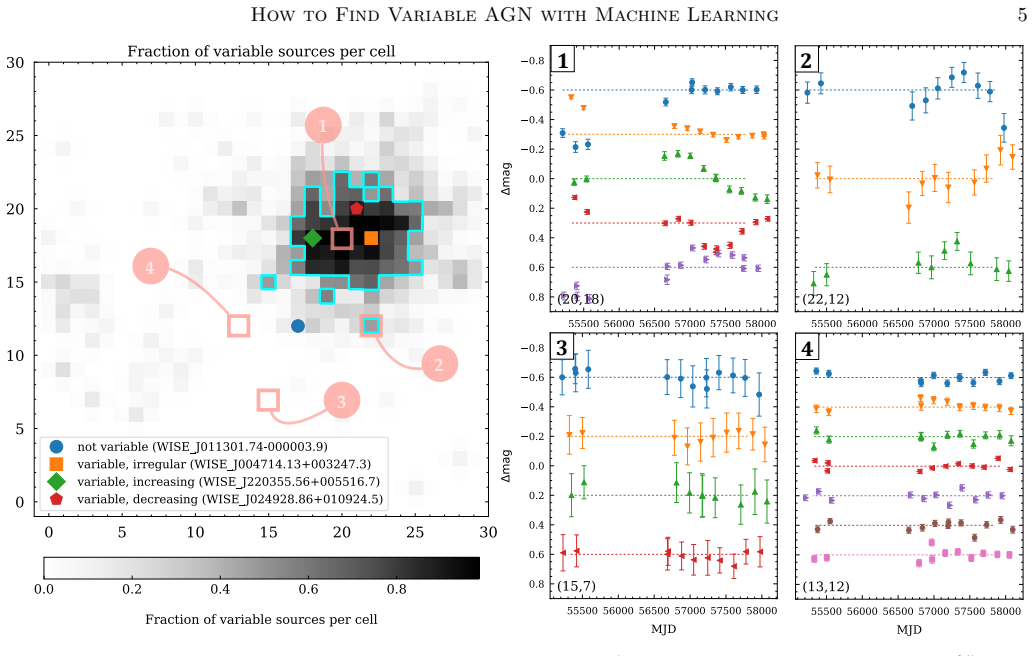
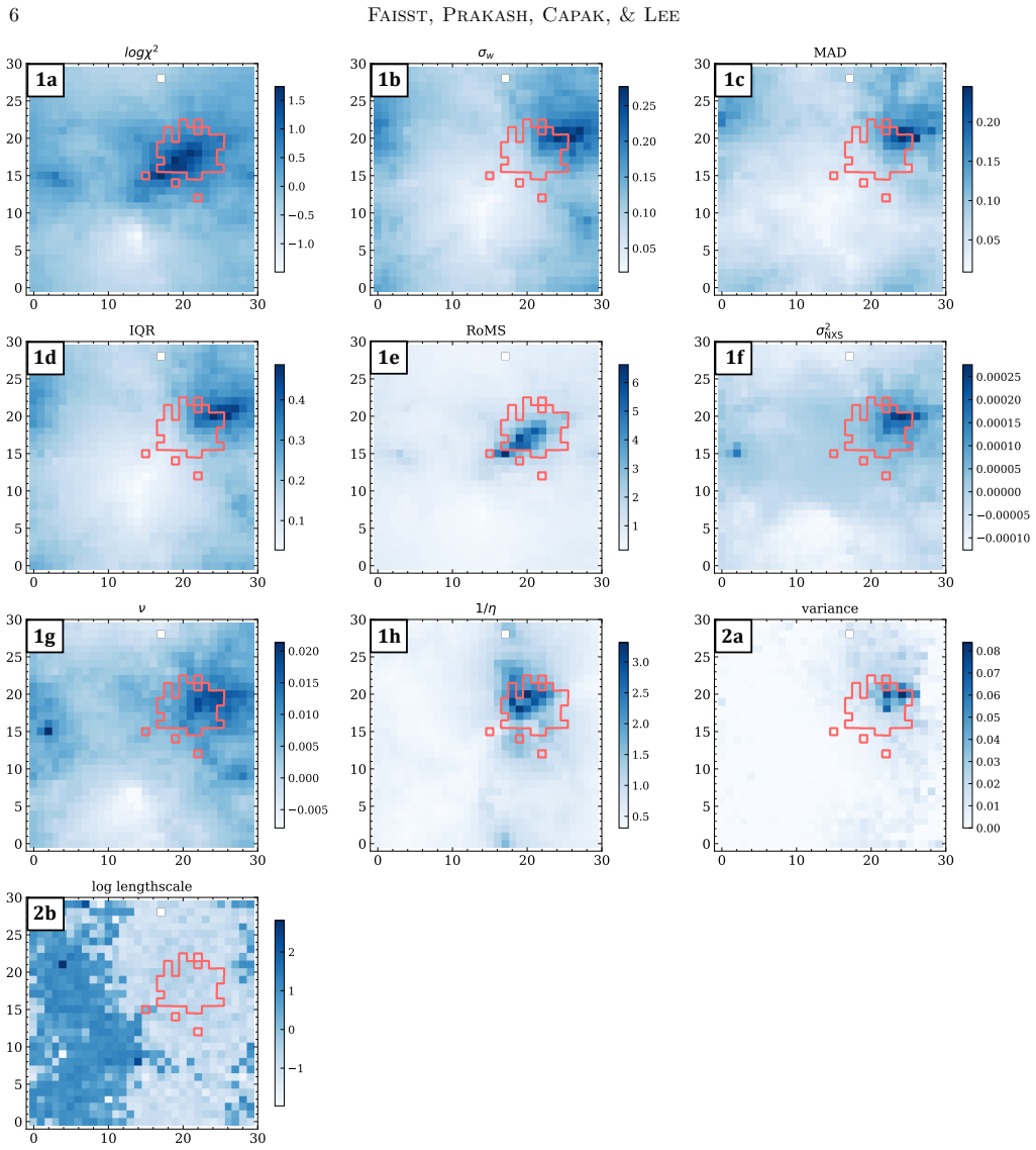
The engine is the self-organizing map, an unsupervised algorithm that folds an N-dimensional feature space into a 30×30 grid of cells while preserving neighborhoods: nearby cells contain light curves with similar variability statistics. The features are eight nonparametric variability estimators — χ², standard deviation, median absolute deviation, interquartile range, robust median statistics, normalized excess variance, peak-to-peak amplitude, and the inverse von Neumann ratio (the ratio that uses correlations between consecutive points, high for smooth trends and low for short-timescale jitter) — plus optional Gaussian-process variance and length-scale parameters. Each cell is labeled variable if more than half of the training light curves mapped into it are variable, and any new light curve is classified instantly by landing in a cell. The cell structure carries the argument: it separates variable from nonvariable objects spatially, and its per-cell median estimator values reveal which statistics track variability and where low signal-to-noise degeneracies hide.
What would settle it
Have two or more independent observers, blind to the original labels, reclassify a random subset of the 8,309 WISE light curves, then retrain and evaluate the SOM against the consensus labels; if purity and completeness fall substantially below 86% and 66%, part of the reported performance is agreement with label noise. A complementary check would inject simulated variable light curves with known amplitudes into the real sample and measure how recovery depends on amplitude.
Extended reading notes
Core claim
The central claim is that a self-organizing map trained on nonparametric variability estimators identifies visually classified variable AGN light curves in a WISE-selected Stripe 82 sample about as well as supervised deep learning, while keeping the data structure visible. Applied to 8,309 AGN candidates, 751 of which were visually flagged as variable, the SOM yields 86% purity and 66% completeness (accuracy 0.94, F1 0.75, Matthews correlation coefficient 0.72); the multilayer-perceptron comparison gives 79% purity and 58% completeness (MCC 0.65). The authors first test the method on simulated light curves with realistic noise and time sampling, where it reaches 91% purity and 79% completeness, then show that on real data the variable curves cluster in a compact region of the map. They also report that separating the three visual subclasses is not robust, a difficulty they attribute to the small size of the monotonic subgroups (66 increasing and 98 decreasing out of 8,309 objects), and that χ², robust median statistics, and the inverse von Neumann ratio carry most of the discriminative signal, while median absolute deviation, interquartile range, and normalized excess variance show degeneracies at low signal-to-noise.
Load-bearing premise
The load-bearing premise is that the visual inspection that sorted 7,558 light curves as nonvariable and 751 as variable provides reliable ground truth; if that labeling is noisy or biased, the purity and completeness numbers measure agreement with the labels rather than real variability detection.
Editorial extensions
If this is right
- The same trained map can classify new light curves instantly without retraining, making it practical for real-time filtering in large time-domain surveys.
- Because it consumes generic variability estimators rather than AGN-specific features, the method is claimed to transfer to supernovae, exoplanet transits, pulsars, and other time-sampled transients.
- The map's cell layout is a built-in diagnostic: per-cell estimator maps expose which variability indicators are reliable and where photometric noise mimics variability, information a deep network does not expose.
- The SOM organizes data without requiring complete labels, so sparse visual classifications can be layered on top of the map rather than used to train a supervised model from scratch.
- On the WISE sample, a variable-AGN catalog selected at the SOM's 86% purity would contain roughly one nonvariable interloper for every six variable objects, a contamination level the authors treat as acceptable for statistical studies.
Reading between the lines
- Because the evaluation labels come from a single visual inspection, the reported 86% and 66% are best read as agreement with those human labels; an independent relabeling study would reveal how much of the apparent performance is shared label noise.
- The estimator maps suggest that χ², RoMS, and the inverse von Neumann ratio dominate the signal while MAD, IQR, and excess variance are degenerate at low signal-to-noise; replacing them with uncertainty-aware estimators could plausibly raise completeness above 66% without sacrificing much purity.
- The per-cell variable fraction is effectively a continuous score, so a survey could threshold it at values other than 50% to trade purity against completeness depending on whether it needs a clean sample or a complete census.
- The same machinery could be extended to multi-band light curves, where the map topology would show whether variability in different wavelengths traces the same cells or separates by physical mechanism.
Signed reviews
Editorial analysis
A structured set of objections, weighed in public.
Referee Report
Summary. The paper presents an unsupervised machine-learning pipeline for identifying variable AGN light curves. The authors define eight nonparametric and two parametric variability estimators, train a self-organizing map (SOM) on an 80% subsample of 8,309 WISE-selected AGN from Stripe 82, and evaluate on the remaining 20%, using a single human visual classification (7,558 nonvariable, 751 variable) as ground truth. On simulated light curves with realistic noise and sampling, the SOM achieves purity 91% and completeness 79%; on the observed sample it is reported to achieve purity 86% and completeness 66% (Eq. 8) with ACC = 0.94, MCC = 0.72, F1 = 0.75. The SOM is compared with a supervised multilayer perceptron, which yields purity 79% and completeness 58%, and the authors conclude that the SOM is comparable while additionally providing visualization of estimator correlations.
Significance. If the reported performance is unbiased, the paper provides a useful, domain-aware alternative to supervised deep learning for variability selection, with fast classification and the ability to visualize correlations on the SOM. The train/test split, the noise-matched simulations, and the comparison to a deep network are strengths, and the use of standard public libraries improves reproducibility. However, the headline numbers are only as good as the visual labels used for training and evaluation, so the current contribution is best read as reproducing a human visual classification; the paper's broader physical claim requires independent validation of those labels.
major comments (3)
- [Section 3.2.2, Eq. (8)] The quoted metrics do not follow from the printed confusion matrix. With C_SOM = ((0.85, 0.01), (0.04, 0.09)), purity is TP/(TP+FP) = 0.09/(0.09+0.01) = 0.90 and completeness is TP/(TP+FN) = 0.09/0.13 = 0.69, not 86% and 66%; MCC also evaluates to about 0.76, not 0.72. The same discrepancy occurs in Eq. (7), Eq. (9), and Eq. (10). Since these numbers are the central quantitative claim, the matrices and quoted metrics must be reconciled (or exact, unrounded values and a rounding policy provided) before the performance can be assessed.
- [Section 2.1 and Section 3.2.2] The ground truth is a single human visual classification of 7,558 nonvariable and 751 variable light curves, with no inter-rater reliability check, no quantitative definition of 'visually variable,' and no independent confirmation. Because the SOM is trained, thresholded, and evaluated against these labels, Eq. (8) measures agreement with this one human classification rather than necessarily detecting physical AGN variability. The simulation test in Section 3.2.1 uses sinusoidal and flat light curves and therefore cannot diagnose systematic biases in the human labels. The authors should either provide an inter-rater reliability assessment, validate against an independent variability indicator, or explicitly restrict the claim to reproducing the visual classification.
- [Section 3.2.1 and Section 3.2.2] The 50% per-cell fraction is described as chosen to 'maximize the metrics,' and the clipping of 100 training objects is retained because it 'improves the performance slightly.' If these choices are made using the held-out test-set metrics, the reported ACC, MCC, purity, and completeness in Eqs. (7) and (8) are not unbiased generalization estimates. A separate validation set should be used for threshold and preprocessing choices, or the sensitivity of the metrics to these choices should be quantified and reported.
minor comments (4)
- [Introduction] In the second paragraph, 'enables the study the formation' should be 'enables the study of the formation,' and 'occurance' should be 'occurrence.'
- [Section 3.3] The optimizer name 'adams' should be 'Adam.'
- [Section 3.2.2] No uncertainty is quoted for the observed purity and completeness; the authors report ±0.01 variation for simulations and should state whether the observed values come from a single SOM run and provide a variance estimate.
- [Section 2.2] The parametric GP estimators are stated to be non-repeatable in about 5% of cases, but the paper does not say whether the variance-estimator results in Section 3.2.2 are from single runs or averaged, which limits reproducibility.
Circularity Check
Minor operating-point tuning on the evaluation data; the central SOM classification is not circular.
-
fitted input called prediction
[Section 3.2.1, paragraph following Eq. 7]
"Each test light curve gets assigned to a SOM-cell and is then classified as variable if more than 50% of the light curves from the training sample in that cell are variable. This choice of fraction maximizes the metrics and is therefore used throughout this work."
The 50% per-cell classification threshold is chosen by maximizing the same purity/completeness metrics that are later reported as the headline results (Eqs. 7 and 8). If this maximization is done on the test sample, the quoted metrics are partly a fitted operating point rather than an unbiased prediction: the threshold is selected to optimize the reported numbers on the data used to compute them. The effect is bounded because the underlying classifier is still a trained SOM over variability estimators, so the central result does not reduce to a definition, but the evaluation is mildly leaked.
full rationale
The paper's central derivation is self-contained rather than circular. The SOM is trained on nonparametric variability estimators, evaluated on a held-out 20% test split in the simulations, and the observed-sample confusion matrix of Eq. 8 is a measured agreement with the visually assigned labels, not a quantity forced by the estimators by construction. The simulation test (Eq. 7) provides independent external validation with known truth, and the deep-learning comparison uses the same training and test setup, so the headline comparison is fair. The visual-classification ground truth is not independently validated, but this is a measurement-validity concern rather than a circularity, because the paper's claims are explicitly about recovering 'these variable classified AGN' and do not assert an independent physical ground truth. The self-citations (for example Masters et al. 2015 and Prakash et al. 2019) are used for method review and sample description, not as load-bearing evidence for the performance claim. The only mild circular step is the selection of the 50% threshold by maximizing the reported metrics, which may leak test information into the operating point; this is a minor evaluation weakness, not a derivation that reduces to its own inputs.
Assumptions & free parameters
free parameters (5)
- SOM grid size =
30x30 cells
- SOM training iterations =
200
- Initial learning rate =
0.05
- Per-cell classification threshold =
50% variable fraction
- Training-sample clipping cut =
Top 1% of any estimator
assumptions (3)
- domain assumption Visual classification provides reliable ground truth for variability.
- domain assumption Nonparametric variability estimators from Sokolovsky et al. (2017) adequately capture variability.
- domain assumption Simulated sinusoidal light curves match the noise and sampling of real WISE observations.
Cite this review
Pith. "Pith review of How to Find Variable Active Galactic Nuclei with Machine Learning." pith.science (2026). https://pith.science/paper/OFUCFGTR
@misc{pith2026190807542,
  author       = {Pith},
  title        = {Pith review of: How to Find Variable Active Galactic Nuclei with Machine Learning},
  year         = {2026},
  howpublished = {\url{https://pith.science/paper/OFUCFGTR}},
  note         = {Machine review of arXiv:1908.07542}
}
read the original abstract
Machine-learning (ML) algorithms will play a crucial role in studying the large datasets delivered by new facilities over the next decade and beyond. Here, we investigate the capabilities and limits of such methods in finding galaxies with brightness-variable active galactic nuclei (AGN). Specifically, we focus on an unsupervised method based on self-organizing maps (SOM) that we apply to a set of nonparametric variability estimators. This technique allows us to maintain domain knowledge and systematics control while using all the advantages of ML. Using simulated light curves that match the noise properties of observations, we verify the potential of this algorithm in identifying variable light curves. We then apply our method to a sample of ~8300 WISE color-selected AGN candidates in Stripe 82, in which we have identified variable light curves by visual inspection. We find that with ML we can identify these variable classified AGN with a purity of 86% and a completeness of 66%, a performance that is comparable to that of more commonly used supervised deep-learning neural networks. The advantage of the SOM framework is that it enables not only a robust identification of variable light curves in a given dataset, but it is also a tool to investigate correlations between physical parameters in multi-dimensional space - such as the link between AGN variability and the properties of their host galaxies. Finally, we note that our method can be applied to any time-sampled light curve (e.g., supernovae, exoplanets, pulsars, and other transient events).
Figures


Figures from the paper (1 more)
Reference graph
Works this paper leans on
-
[1]
2019, MNRAS, 482, 5078
Aguirre, C., Pichara, K., & Becker, I. 2019, MNRAS, 482, 5078
2019
-
[2]
J., Pollacco, D., & Santerne, A
Armstrong, D. J., Pollacco, D., & Santerne, A. 2017, MNRAS, 465, 2634
work page 2017
-
[3]
Armstrong, D. J., Kirk, J., Lam, K. W. F., et al. 2016, MNRAS, 456, 2260
work page 2016
-
[4]
Bonjean, V., Aghanim, N., Salom´ e, P., et al. 2019, A&A, 622, A137
work page 2019
-
[5]
G., Benson, A
Bower, R. G., Benson, A. J., Malbon, R., et al. 2006, MNRAS, 370, 645
2006
- [6]
-
[7]
Deep Learning for Image Sequence Classification of Astronomical Events
Carrasco-Davis, R., Cabrera-Vives, G., F¨ orster, F., et al. 2018, arXiv e-prints, arXiv:1807.03869 Carrasco Kind, M., & Brunner, R. J. 2014, MNRAS, 438, 3409
work page Pith review arXiv 2018
- [8]
Show all 44 references
-
[9]
2017, ApJ, 837, L28
Charnock, T., & Moss, A. 2017, ApJ, 837, L28
2017
-
[10]
J., Springel, V., White, S
Croton, D. J., Springel, V., White, S. D. M., et al. 2006, MNRAS, 365, 11
2006
-
[11]
L., et al
Davidzon, I., Laigle, C., Capak, P. L., et al. 2019, arXiv e-prints, arXiv:1905.13233
2019 arXiv
-
[12]
2013, MNRAS, 433, 3297
Dubois, Y., Gavazzi, R., Peirani, S., & Silk, J. 2013, MNRAS, 433, 3297
2013
-
[13]
S., Pacholczyk, A
Fitch, W. S., Pacholczyk, A. G., & Weymann, R. J. 1967, ApJL, 150, L67
1967
-
[14]
O., Sederberg, P
Hanke, M., Halchenko, Y. O., Sederberg, P. B., et al. 2009, Neuroinformatics, 7, 37
2009
-
[15]
2019a, arXiv e-prints, arXiv:1905.10379
Hemmati, S., Capak, P., Pourrahmani, M., et al. 2019a, arXiv e-prints, arXiv:1905.10379
1905 arXiv
-
[16]
A., Tat, K., & Thorp, R
Hinners, T. A., Tat, K., & Thorp, R. 2018, AJ, 156, 7
2018
-
[17]
2012, MNRAS, 420, 320
Hernquist, L. 2012, MNRAS, 420, 320
2012
-
[18]
2014, ApJS, 213, 12
Jiang, L., Fan, X., Bian, F., et al. 2014, ApJS, 213, 12
2014
-
[19]
Kawaguchi, T., Mineshige, S., Umemura, M., & Turner, E. L. 1998, ApJ, 504, 671
1998
-
[20]
1982, Biological Cybernetics, 43, 59
Kohonen, T. 1982, Biological Cybernetics, 43, 59
1982
-
[21]
1990, IEEE, 78, 1464 How to Find V ariable AGN with Machine Learning 9
Kohonen, T. 1990, IEEE, 78, 1464 How to Find V ariable AGN with Machine Learning 9
1990
-
[22]
2016, A&A, 596, A39
Krakowski, T., Ma lek, K., Bilicki, M., et al. 2016, A&A, 596, A39
2016
-
[23]
Winter, M. K. 2016, ApJS, 225, 31
2016
-
[24]
2011, ApJ, 731, 53
Mainzer, A., Bauer, J., Grav, T., et al. 2011, ApJ, 731, 53
2011
-
[25]
2015, ApJ, 813, 53
Masters, D., Capak, P., Stern, D., et al. 2015, ApJ, 813, 53
2015
-
[26]
C., Stern, D
Masters, D. C., Stern, D. K., Cohen, J. G., et al. 2019, ApJ, 877, 81
2019
-
[27]
1975, Biochimica et Biophysica Acta (BBA) - Protein Structure, 405, 442
Matthews, B. 1975, Biochimica et Biophysica Acta (BBA) - Protein Structure, 405, 442
1975
-
[28]
S., Biswas, R., & Hloˇ zek, R
Muthukrishna, D., Narayan, G., Mandel, K. S., Biswas, R., & Hloˇ zek, R. 2019a, arXiv e-prints, arXiv:1904.00014
1904 arXiv
-
[29]
2019b, arXiv e-prints, arXiv:1903.02557
Muthukrishna, D., Parkinson, D., & Tucker, B. 2019b, arXiv e-prints, arXiv:1903.02557
1903 arXiv
-
[30]
B., & Gunn, J
Oke, J. B., & Gunn, J. E. 1983, ApJ, 266, 713
1983
-
[31]
Peterson, B. M. 1997, An Introduction to Active Galactic Nuclei
1997
-
[32]
R., Helou, G., et al
Prakash, A., Chary, R. R., Helou, G., et al. 2019, arXiv e-prints, arXiv:1908.04280
2019 arXiv
-
[33]
O., Norris, R
Ralph, N. O., Norris, R. P., Fang, G., et al. 2019, arXiv e-prints, arXiv:1906.02864
2019 arXiv
-
[34]
Rampone, S., Pierro, V., Troiano, L., & Pinto, I. M. 2013, International Journal of Modern Physics C, 24, 1350084
2013
-
[35]
2017, AJ, 153, 204
Sesar, B., Hernitschek, N., Mitrovi´ c, S., et al. 2017, AJ, 153, 204
2017
-
[36]
Shields, G. A. 1978, in BAAS, Vol. 10, Bulletin of the American Astronomical Society, 690
1978
-
[37]
2007, MNRAS, 380, 877
Sijacki, D., Springel, V., Di Matteo, T., & Hernquist, L. 2007, MNRAS, 380, 877
2007
-
[38]
2018, A&A, 617, A70
Siudek, M., Ma lek, K., Pollo, A., et al. 2018, A&A, 617, A70
2018
-
[39]
V., Gavras, P., Karampelas, A., et al
Sokolovsky, K. V., Gavras, P., Karampelas, A., et al. 2017, MNRAS, 464, 274
2017
-
[40]
A., et al
Sooknunan, K., Lochner, M., Bassett, B. A., et al. 2018, arXiv e-prints, arXiv:1811.08446
2018 arXiv
-
[41]
J., Benford, D
Stern, D., Assef, R. J., Benford, D. J., et al. 2012, ApJ, 753, 30
2012
-
[42]
2008, A&A, 482, 483
Torniainen, I., Tornikoski, M., Turunen, M., et al. 2008, A&A, 482, 483
2008
-
[43]
S., Baldry, I
Turner, S., Kelvin, L. S., Baldry, I. K., et al. 2019, MNRAS, 482, 126
2019
-
[44]
L., Eisenhardt, P
Wright, E. L., Eisenhardt, P. R. M., Mainzer, A. K., et al. 2010, AJ, 140, 1868
2010
Reviewed August 14, 2026 · model on record in the stance chip above.
Discussion (0). Continue with ORCID to comment.