REVIEW 2 major objections 3 minor 37 references
Iterative Linearized Control: Stable Algorithms and Complexity Guarantees
T0 review · 2 major / 3 minor · reviewed 2026-08-14 · deepseek-v4-flash
Pith's one-line read Regularized ILQR converges in O(1/epsilon^2) iterations
desk verdict First worst-case complexity bounds for ILQR-style control, with a small but repairable gap in the main line-search constant and a conditional accelerated rate. read the letter →
The pith
A machine-rendered reading of the paper's core claim, the machinery that carries it, and where it could break.
The reading
What carries the argument
The load-bearing object is the regularized Gauss-Newton step (37), $\bar u_{k+1}=\bar u_k+\arg\min_{\bar v}\{c_f(\bar u_k+\bar v;\bar u_k)+(2\gamma_k)^{-1}\|\bar v\|^2\}$, with the convex model $c_f(\bar v;\bar u)=h(\tilde x(\bar u)+\nabla\tilde x(\bar u)^\top(\bar v-\bar u))+g(\bar v)$. For quadratic $h$ and $g$ this reduces to ILQR plus a proximal penalty and admits the closed form $\bar u_{k+1}=\bar u_k-(\nabla\tilde x(\bar u_k)H\nabla\tilde x(\bar u_k)^\top+G+\gamma_k^{-1}I)^{-1}\nabla f(\bar u_k)$, which is what links iterate differences to gradient norms. The supporting mechanism is the equivalence (Propositions 2.1–2.3 and 3.6) between dynamic programming for the linear-quadratic subproblem and calls to an automatic-differentiation oracle, so that the oracle count is a faithful measure of computational cost.
What would settle it
On a smooth composite control example with known smoothness constants and suboptimality gap, run the regularized Gauss-Newton method (37) with the decreasing line-search of Algorithm 13 and measure the smallest $N$ with $\|\nabla f(\bar u_N)\le\varepsilon$ for several $\varepsilon$; if the count grows faster than $2L(f(\bar u_0)-f_*)/\varepsilon^2$ (up to the logarithmic line-search term), Corollary 4.4 is contradicted. To test the accelerated claim, evaluate $\min_{\bar u,\bar v}(f(\bar v)-c_f(\bar v;\bar u))$ on a concrete convex-composite instance; if this minimum is strictly negative while the algorithm still shows a $1/N^2$ objective decrease, then the lower-bound hypothesis (42) is not necessary for the observed speed-up.
Extended reading notes
Core claim
The central claim is that iterative linearization control—ILQR in exact dynamics and ILQG in noisy dynamics—is best understood as model-minimization on the composite objective $f(\bar u)=h(\tilde x(\bar u))+g(\bar u)$, and that the model-minimization subproblem is a linear-quadratic control problem solvable by dynamic programming in time linear in the horizon $\tau$. The paper's main new result is that augmenting the ILQR model with a proximal term $(2\gamma_k)^{-1}\|\bar u-\bar u_k\|^2$ gives the regularized Gauss-Newton method (37), which with a decreasing line-search finds an $\varepsilon$-stationary point in at most $O(1/\varepsilon^2)$ calls to the regularized Gauss-Newton oracle (Corollary 4.4). It further shows that the accelerated variant in Algorithm 1 preserves this guarantee and, under the extra assumption that the convex model satisfies $c_f(\bar v;\bar u)\le f(\bar v)$ for all $\bar u,\bar v$—an assumption that forces $f$ to be convex—achieves $f(\bar u_N)-f_*\le 4\delta^{-1}\|\bar u^*-\bar u_0\|^2/(N+1)^2$ (Proposition 4.5).
Load-bearing premise
The accelerated $O(1/N^2)$ rate rests on the assumption that the convex model $c_f(\bar v;\bar u)$ never exceeds the true objective $f(\bar v)$, which forces $f$ to be convex; if that fails, the paper only claims the slower $O(1/N)$ stationary-point rate.
Editorial extensions
If this is right
- Corollary 4.4 gives a worst-case oracle complexity for an ILQR-type method: $O(1/\varepsilon^2)$ calls to the regularized Gauss-Newton oracle for an $\varepsilon$-stationary point of the composite control objective.
- Corollary 4.6 turns this into automatic-differentiation oracle complexity: for problems with a final-state cost the regularized method needs $(2d+1)$ times the Gauss-Newton count, so the proximal fix costs only a constant factor over a gradient step.
- The model-minimization viewpoint unifies gradient descent, Gauss-Newton, and Levenberg-Marquardt for control: all are linear-quadratic control solves, hence all cost roughly the same as one gradient computation in the horizon length $\tau$.
- The accelerated Algorithm 1 inherits the non-accelerated guarantee and, when the convex model lower-bounds the objective (which forces convexity), converges at rate $O(1/N^2)$ in objective value.
Reading between the lines
- A direct extension the paper leaves open: the rollout-based iLQG/DDP variant is not analyzed, but the same proximal-regularization template would likely endow it with the same $O(1/\varepsilon^2)$ guarantee; that is an inference, not a paper claim.
- The automatic-differentiation/dynamic-programming equivalence points beyond control: any nested composition with a convex quadratic outer cost and smooth inner maps is a candidate for the same regularized Gauss-Newton complexity analysis.
- The lower-bound condition (42) suggests a practical design rule for model-based optimization: if the surrogate model underestimates the true cost, acceleration is provable; if not, the safe choice is the non-accelerated proximal step.
Signed reviews
Editorial analysis
A structured set of objections, weighed in public.
Referee Report
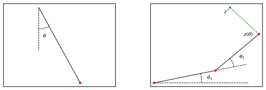
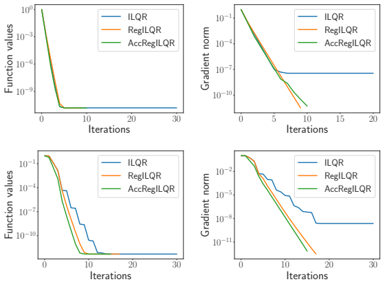
Summary. The manuscript studies finite-horizon discrete-time nonlinear control through the lens of composite optimization. It reformulates the control objective as f(\bar u)=h(\tilde x(\bar u))+g(\bar u), identifies the relevant automatic-differentiation oracle, and shows that dynamic-programming steps for linear-quadratic subproblems are equivalent to gradient back-propagation. The main results are a regularized Gauss-Newton method (regularized ILQR) with a claimed O(1/epsilon^2) iteration complexity to epsilon-stationarity (Corollary 4.4) and an accelerated variant with a claimed O(1/N^2) rate under a model lower-bound condition (Proposition 4.5). The paper also gives oracle-cost comparisons, PyTorch experiments on a pendulum and a two-link arm, and a public code repository.
Significance. If the proofs are completed, the paper gives the first worst-case complexity guarantee for ILQR-type algorithms, expressed in calls to an automatic-differentiation oracle, and it usefully connects DDP/ILQR to first-order composite optimization. The derivations of the oracle costs and of the DP/back-propagation equivalence are clean and practically relevant, and the release of code is a concrete strength. The central non-accelerated analysis is standard in structure, but as written it is not fully supported by the line-search in the appendix; the gap is localized and repairable rather than fatal.
major comments (2)
- [§4.2, Cor. 4.4 and Appendix E, Algo. 13–14] The line-search that supports Corollary 4.4 is not the line-search analyzed in the theorem. Condition (39) and Prop. 4.1 use f(\bar u_{k+1}) ≤ c_f(\bar u_{k+1};\bar u_k) + (1/(2γ_k))\|\bar u_{k+1}-\bar u_k\|^2, while Algorithms 13 and 14 use γ_k/2 in the same place. Under the γ_k/2 version, the strong-convexity subtraction in the proof of Prop. 4.1 cannot be combined with the line-search condition to obtain the claimed descent inequality. In addition, Algorithm 13 has no lower bound on the accepted step size: after a rejection above γ̂, the loop may accept γ < γ̂. Since Lemma 4.3 only shows that every γ ≤ γ̂ satisfies (39), this situation is possible. The constant L in Cor. 4.4 is maximized over [γ̂, γ0], so for accepted γ < γ̂ the bound from Prop. 4.1 may fail; with ℓ^2_{\tilde x,S}L_h+L_g = 1, γ̂ = 0.1, γ0 = 0.2, and γ = 0.05, one obtains γ(A+γ^{-1})^2 ≈ 22.0, whereas the maximum over [0.1,0.2] is about 12.0. The theorem can be repaired by flooring the line-search at γ̂ and by consistently using (2γ_k)^{-1} in the pseudocode, or by restating L over the accepted range [min_k γ_k, γ0]. As printed, the proof of the central O(1/ε^2) guarantee does not go through for the algorithm stated.
- [§4.3, Prop. 4.5, Eq. (42)] The O(1/N^2) rate is contingent on the model lower-bound condition c_f(\bar v;\bar u) ≤ f(\bar v) for all \bar u,\bar v. As the proof immediately notes, this condition implies convexity of f (via Lemma 8.3 of Drusvyatskiy and Paquette). This is a strong structural assumption, not a minor technicality: it is exactly what converts the Catalyst extrapolation into a genuinely faster rate. The paper should state in the abstract and in Section 4.3 that the accelerated rate applies to convex-composite objectives satisfying (42), and that no accelerated worst-case rate is claimed for the general nonlinear control problems used in the experiments. As it stands, the presentation invites the reader to attribute the accelerated guarantee to the algorithm at large.
minor comments (3)
- [§5.2] The experiments use a constant step-size tuned after a burn-in phase; they do not exercise the backtracking line-search of Cor. 4.4, so the reported speedup of the accelerated variant is empirical only. A sentence making this explicit would avoid over-reading the plots.
- [§2.2, Prop. 2.4] The assumption that ∇²_xx φ_t, ∇²_xw φ_t, and ∇²_ux φ_t vanish is stated without discussion; a brief remark on how restrictive this is for the noisy-dynamics model would help, since the noisy analysis is not part of the Cor. 4.4 guarantee.
- [§4.2, Eq. (41)] The threshold γ̂ depends on ℓ_{f,S} and M_C, which are not computable in practice; the paper should say explicitly that the guarantee is existential and that the theory does not prescribe a concrete initial step-size γ0.
Circularity Check
Not circular: the complexity bounds are derived from stated smoothness and regularity assumptions together with prior external optimization results, and no fitted quantity is renamed as a prediction.
full rationale
The paper's central claim, Corollary 4.4, is a direct consequence of Proposition 4.1, Lemma 4.2, and Lemma 4.3, all of which are proved in the paper from explicit assumptions on the objective and dynamics. The constant L in the bound is defined from problem data (smoothness constants, the Lipschitz constant of the trajectory map, and the step-size range) and is not fitted to experimental output. No experimental step-size or burn-in phase enters the theoretical bound, so no fitted input is relabeled as a prediction. The accelerated statement in Proposition 4.5 invokes Lemma 8.3 of Drusvyatskiy and Paquette and Lemma B.1 of Paquette et al.; these are prior works co-authored by two of the present authors, but they are external published technical lemmas with stated assumptions, and the present proof does not reduce to a self-citation chain that smuggles in the target result. The reformulation of ILQR as a regularized Gauss-Newton method is an interpretation grounded in the paper's own equations, not a renaming that carries the convergence result by definition. The possible concern that the line-search in Corollary 4.4 may accept step-sizes below gamma-hat is a correctness gap about the proof's constant, not a circularity: the derivation is self-contained and does not assume what it proves.
Assumptions & free parameters
free parameters (2)
- Regularization step-size gamma for RegILQR/AccRegILQR in experiments =
not reported numerically; tuned after 5-iteration burn-in
- Initial step-size gamma_0 and decreasing factor rho in backtracking line-search =
gamma_0 >= gammahat arbitrary; 0 < rho < 1
assumptions (3)
- domain assumption The dynamics phi_t and costs h_t, g_t are sufficiently smooth (differentiable, with Lipschitz continuous gradients on compact sets).
- ad hoc to paper The convex model c_f(v; u) lower bounds the objective f everywhere (Eq. 42) to obtain the accelerated O(1/N^2) rate.
- ad hoc to paper For the noisy dynamics analysis, the second derivatives nabla^2_xx phi_t, nabla^2_xw phi_t, and nabla^2_ux phi_t are zero (Prop 2.4).
Cite this review
Pith. "Pith review of Iterative Linearized Control: Stable Algorithms and Complexity Guarantees." pith.science (2026). https://pith.science/paper/POHVSHDY
@misc{pith2026190807615,
  author       = {Pith},
  title        = {Pith review of: Iterative Linearized Control: Stable Algorithms and Complexity Guarantees},
  year         = {2026},
  howpublished = {\url{https://pith.science/paper/POHVSHDY}},
  note         = {Machine review of arXiv:1908.07615}
}
read the original abstract
We examine popular gradient-based algorithms for nonlinear control in the light of the modern complexity analysis of first-order optimization algorithms. The examination reveals that the complexity bounds can be clearly stated in terms of calls to a computational oracle related to dynamic programming and implementable by gradient back-propagation using machine learning software libraries such as PyTorch or TensorFlow. Finally, we propose a regularized Gauss-Newton algorithm enjoying worst-case complexity bounds and improved convergence behavior in practice. The software library based on PyTorch is publicly available.
Figures
Reference graph
Works this paper leans on
-
[1]
Abadi, M., Agarwal, A., Barham, P., Brevdo, E., Chen, Z., Citro, C., Corrado, G. S., Davis, A., Dean, J., Devin, M., Ghemawat, S., Goodfellow, I., Harp, A., Irving, G., Isard, M., Jia, Y., Jozefowicz, R., Kaiser, L., Kudlur, M., Levenberg, J., Man\' e , D., Monga, R., Moore, S., Murray, D., Olah, C., Schuster, M., Shlens, J., Steiner, B., Sutskever, I., T...
work page 2015
-
[2]
Introduction to the mathematical theory of control processes, volume 2
Bellman, R. Introduction to the mathematical theory of control processes, volume 2. Academic press, 1971
work page 1971
-
[3]
Bertsekas, D. P. Dynamic programming and optimal control. Athena Scientific, 3rd edition, 2005
work page 2005
-
[4]
Numerical methods for least squares problems
Bjorck, A. Numerical methods for least squares problems. SIAM, 1996
work page 1996
-
[5]
Burke, J. V. Descent methods for composite nondifferentiable optimization problems. Mathematical Programming, 33 0 (3): 0 260--279, 1985
work page 1985
-
[6]
Cartis, C., Gould, N. I. M., and Toint, P. L. On the evaluation complexity of composite function minimization with applications to nonconvex nonlinear programming. SIAM Journal on Optimization, 21 0 (4): 0 1721--1739, 2011
work page 2011
-
[7]
De O. Pantoja, J. Differential dynamic programming and N ewton's method. International Journal of Control, 47 0 (5): 0 1539--1553, 1988
work page 1988
-
[8]
Regret bounds for robust adaptive control of the linear quadratic regulator
Dean, S., Mania, H., Matni, N., Recht, B., and Tu, S. Regret bounds for robust adaptive control of the linear quadratic regulator. In Advances in Neural Information Processing Systems, pp.\ 4188--4197, 2018
work page 2018
Show all 37 references
-
[9]
L., Huang, M., Kolmanovsky, I
Dontchev, A. L., Huang, M., Kolmanovsky, I. V., and Nicotra, M. M. Inexact N ewton- K antorovich methods for constrained nonlinear model predictive control. IEEE Transactions on Automatic Control, 2018
2018
-
[10]
and Paquette, C
Drusvyatskiy, D. and Paquette, C. Efficiency of minimizing compositions of convex functions and smooth maps. Mathematical Programming, pp.\ 1--56, 2018
2018
-
[11]
Dunn, J. C. and Bertsekas, D. P. Efficient dynamic programming implementations of N ewton's method for unconstrained optimal control problems. Journal of Optimization Theory and Applications, 63 0 (1): 0 23--38, 1989
1989
-
[12]
Global convergence of policy gradient methods for the linear quadratic regulator
Fazel, M., Ge, R., Kakade, S., and Mesbahi, M. Global convergence of policy gradient methods for the linear quadratic regulator. In Proceedings of the 35th International Conference on Machine Learning, volume 80, 2018
2018
-
[13]
and Walther, A
Griewank, A. and Walther, A. Evaluating derivatives: principles and techniques of algorithmic differentiation. SIAM, 2008
2008
-
[14]
and Pannek, J
Gr \"u ne, L. and Pannek, J. Nonlinear model predictive control. Springer, 2017
2017
-
[15]
C., Pereyra, V., and Scherer, G
Hansen, P. C., Pereyra, V., and Scherer, G. Least squares data fitting with applications. JHU Press, 2013
2013
-
[16]
Jacobson, D. H. and Mayne, D. Q. Differential Dynamic Programming. Elsevier, 1970
1970
-
[17]
Kakade, S. M. and Lee, J. D. Provably correct automatic sub-differentiation for qualified programs. In Advances in Neural Information Processing Systems, pp.\ 7125--7135, 2018
2018
-
[18]
Iterative regularization methods for nonlinear ill-posed problems, volume 6
Kaltenbacher, B., Neubauer, A., and Scherzer, O. Iterative regularization methods for nonlinear ill-posed problems, volume 6. Walter de Gruyter, 2008
2008
-
[19]
A theoretical framework for back-propagation
LeCun, Y., Touresky, D., Hinton, G., and Sejnowski, T. A theoretical framework for back-propagation. In Proceedings of the 1988 connectionist models summer school, volume 1, pp.\ 21--28, 1988
1988
-
[20]
Lewis, A. S. and Wright, S. J. A proximal method for composite minimization. Mathematical Programming, 158: 0 501--546, 2016
2016
-
[21]
and Todorov, E
Li, W. and Todorov, E. Iterative linear quadratic regulator design for nonlinear biological movement systems. In 1st International Conference on Informatics in Control, Automation and Robotics, volume 1, pp.\ 222--229, 2004
2004
-
[22]
and Todorov, E
Li, W. and Todorov, E. Iterative linearization methods for approximately optimal control and estimation of non-linear stochastic system. International Journal of Control, 80 0 (9): 0 1439--1453, 2007
2007
-
[23]
and Shoemaker, C
Liao, L.-Z. and Shoemaker, C. A. Convergence in unconstrained discrete-time differential dynamic programming. IEEE Transactions on Automatic Control, 36 0 (6): 0 692--706, 1991
1991
-
[24]
and Shoemaker, C
Liao, L.-Z. and Shoemaker, C. A. Advantages of differential dynamic programming over N ewton's method for discrete-time optimal control problems. Technical report, Cornell University, 1992
1992
-
[25]
A second-order gradient method for determining optimal trajectories of non-linear discrete-time systems
Mayne, D. A second-order gradient method for determining optimal trajectories of non-linear discrete-time systems. International Journal of Control, 3 0 (1): 0 85--95, 1966
1966
-
[26]
Modified G auss- N ewton scheme with worst case guarantees for global performance
Nesterov, Y. Modified G auss- N ewton scheme with worst case guarantees for global performance. Optimization Methods & Software, 22 0 (3): 0 469--483, 2007
2007
-
[27]
and Wright, S
Nocedal, J. and Wright, S. J. Numerical Optimization. Springer, 2nd edition, 2006
2006
-
[28]
Catalyst for gradient-based nonconvex optimization
Paquette, C., Lin, H., Drusvyatskiy, D., Mairal, J., and Harchaoui, Z. Catalyst for gradient-based nonconvex optimization. In 21st International Conference on Artificial Intelligence and Statistics, pp.\ 1--10, 2018
2018
-
[29]
Automatic differentiation in P y T orch, 2017
Paszke, A., Gross, S., Chintala, S., Chanan, G., Yang, E., DeVito, Z., Lin, Z., Desmaison, A., Antiga, L., and Lerer, A. Automatic differentiation in P y T orch, 2017. URL https://pytorch.org/
2017
-
[30]
A tour of reinforcement learning: The view from continuous control
Recht, B. A tour of reinforcement learning: The view from continuous control. Annual Review of Control, Robotics, and Autonomous Systems, 2018
2018
-
[31]
N., and Morari, M
Richter, S., Jones, C. N., and Morari, M. Computational complexity certification for real-time MPC with input constraints based on the fast gradient method. IEEE Transactions on Automatic Control, 57 0 (6): 0 1391--1403, 2012
2012
-
[32]
and Bobrow, J
Sideris, A. and Bobrow, J. E. An efficient sequential linear quadratic algorithm for solving nonlinear optimal control problems. In Proceedings of the American Control Conference, pp.\ 2275--2280, 2005
2005
-
[33]
Synthesis and stabilization of complex behaviors through online trajectory optimization
Tassa, Y., Erez, T., and Todorov, E. Synthesis and stabilization of complex behaviors through online trajectory optimization. In 2012 IEEE/RSJ International Conference on Intelligent Robots and Systems, pp.\ 4906--4913. IEEE, 2012
2012
-
[34]
Control-limited differential dynamic programming
Tassa, Y., Mansard, N., and Todorov, E. Control-limited differential dynamic programming. In IEEE International Conference on Robotics and Automation, pp.\ 1168--1175, 2014
2014
-
[35]
and Li, W
Todorov, E. and Li, W. Optimal control methods suitable for biomechanical systems. In Proceedings of the 25th Annual International Conference of the IEEE, volume 2, pp.\ 1758--1761, 2003
2003
-
[36]
and Li, W
Todorov, E. and Li, W. A generalized iterative lqg method for locally-optimal feedback control of constrained nonlinear stochastic systems. In Proceedings of the American Control Conference, pp.\ 300--306, 2005
2005
-
[37]
Optimization over Time
Whittle, P. Optimization over Time. John Wiley & Sons, Inc., New York, NY, USA, 1982
1982
Reviewed August 14, 2026 · model on record in the stance chip above.
Discussion (0). Continue with ORCID to comment.