Data-driven model reduction, Wiener projections, and the Koopman-Mori-Zwanzig formalism

Fei Lu; Kevin K. Lin

REVIEW 4 major objections 6 minor 78 references

Data-driven model reduction, Wiener projections, and the Koopman-Mori-Zwanzig formalism

T0 review · 4 major / 6 minor · reviewed 2026-08-14 · deepseek-v4-flash

Challenge this review Re-run · record.json Download PDF Read on arXiv ↗ Review JSON

Pith's one-line read A Wiener projection onto the span of a resolved observable and all its pullbacks turns data-driven reduced models into optimal linear filters, with NARMAX as the rational approximation.

desk verdict The Wiener projection cleanly links Koopman-Mori-Zwanzig and NARMAX, but the paper's strongest orthogonality result is proven only for invertible/unitary systems, and the dissipative examples step outside that assumption. read the letter →

arxiv 1908.07725 v5 pith:KR5UUJTT submitted 2019-08-21 math.NA cs.NAphysics.comp-phstat.ML

Kevin K. Lin , Fei Lu This is my paper · ORCID

classification math.NAcs.NAphysics.comp-phstat.ML MSC 37M1060G1093E11

keywords modelreductionWienerprojectionMori-ZwanzigformalismKoopmanoperatorNARMAXnon-MarkoviandynamicsKuramoto-SivashinskyequationstochasticBurgers

verification ladder T0 review T1 audit T2 compute T3 formal

The pith

A machine-rendered reading of the paper's core claim, the machinery that carries it, and where it could break.

The reading

This paper argues that many data-driven reduced models of complex dynamical systems are really the same object: an optimal linear filter in a chosen space of observables, whose transfer function is then approximated by a ratio of polynomials. The authors define a Wiener projection onto the span of the observable map and all its pullbacks under the inverse dynamics, and show it makes the Mori-Zwanzig memory expansion exact with a strong orthogonality condition: the residual noise at each step is uncorrelated with every past observable. From this, the widely used NARMAX model follows as the rational-approximation step, giving such empirical models a dynamical-systems justification. If this picture is right, then fitting a reduced model is not an ad hoc regression but a principled approximation of an optimal filter, and classical Wiener filtering becomes an alternative foundation for model reduction alongside Mori-Zwanzig theory.

What carries the argument

The Wiener projection $P_W$ is the orthogonal projection onto $W = \operatorname{span}(\Psi \cup M^{-1}\Psi \cup M^{-2}\Psi \cup \cdots)$, the closed subspace generated by the vector of resolved observables $\Psi(x)$ and all its preimages under the Koopman operator $M$. Under the assumption that the dynamics map $F$ is invertible, making $M$ unitary on $L^2(\mu)$, the identity $M^{-\ell}P_W = P_W M^{-\ell}P_W$ collapses the Dyson expansion, leaving the exact one-step predictor with the strong orthogonality $\langle \xi_n, \Psi(x_m)\rangle = 0$ for $n>m$. The second piece is the rational-approximation ansatz $H(z)\approx B(z)/A(z)$ for the $z$-transform of the filter coefficients, which turns the infinite convolution into the finite-order NARMAX recursion; the paper enforces the decaying-memory condition by factoring $A(z)$ into second-order blocks, a cascade form whose roots lie inside the unit disc.

What would settle it

Take a strongly dissipative one-dimensional map that is not invertible, run the paper's NARMAX fitting procedure with a fixed observable $\Psi$, and measure the sample covariance between the residuals $\xi_n$ and past observables $\Psi(x_m)$ for $n>m$; if it is significantly nonzero, the strong orthogonality (3.6b) fails and the Wiener-projection derivation does not extend to non-invertible dynamics as claimed.

Watch

Extended reading notes

Core claim

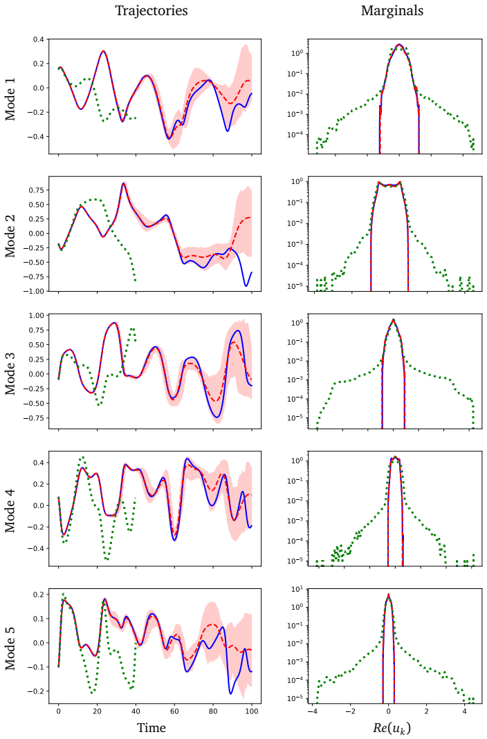
The central discovery is that the orthogonal projection $P_W$ onto $W = \operatorname{span}(\Psi \cup M^{-1}\Psi \cup M^{-2}\Psi \cup \cdots)$, where $\Psi$ collects the resolved observables and $M$ is the Koopman operator, yields the exact decomposition $x_{n+1} = \sum_{k\ge 0} \Psi(x_{n-k})\cdot h_k + \xi_{n+1}$ with $\langle \xi_n, \Psi(x_m)\rangle = 0$ for every $n>m$. This Wiener projection absorbs all memory effects into the subspace $W$, so the Dyson expansion collapses and the residual is orthogonal to the entire past observable history, not just a finite-dimensional subspace as in the usual Mori-Zwanzig projection. Because the coefficients $h_k$ form the impulse response of a causal Wiener filter, replacing its $z$-transform $H(z)$ by a rational function $B(z)/A(z)$ produces a NARMAX-type recursion; the paper calls this the derivation of NARMAX from the underlying dynamics. The result is demonstrated on the Kuramoto-Sivashinsky equation, where the five-mode reduced model reproduces short-time tracking, autocovariances, energy spectra, and energy cross-correlations, and on a stochastically forced viscous Burgers equation, where a nine-mode model forecasts the response of individual forcing realizations.

Load-bearing premise

The entire clean orthogonality and the NARMAX derivation assume the dynamics map $F$ is invertible, so that the Koopman operator $M$ is invertible and unitary; the paper's numerical successes on dissipative systems like Kuramoto-Sivashinsky rest on an asserted, not proved, extension to that case.

Editorial extensions

If this is right

NARMAX models acquire a dynamical-systems derivation: they are rational approximations of the Wiener filter associated with the Koopman–Mori-Zwanzig decomposition, giving a principled reason for their empirical success.
For stationary chaotic and randomly forced systems, the decomposition is exact in law before approximation, so the only modeling choices are the observable map $\Psi$ and the order of the rational approximation.
The strong orthogonality $\langle \xi_n, \Psi(x_m)\rangle = 0$ for $n>m$ provides a least-squares optimality guarantee for reduced models that use only past observables, supporting the common practice of adding independent noise after fitting.
Classical Wiener filtering can serve as an alternative foundation for model reduction alongside Mori-Zwanzig when statistics are time-stationary.
Because the method works with the recent history of $\Psi$, it is formally applicable to dissipative systems without computing the inverse map $F^{-1}$, as demonstrated on the Kuramoto-Sivashinsky and stochastic Burgers equations.

Reading between the lines

Editorial extensions of the paper, not claims the author makes directly.

An editor-level test of the paper's asserted dissipative extension: compute the sample correlation between NARMAX residuals and past observables for a strongly non-invertible map; nonzero values would show the strong orthogonality (3.6b) is not automatic outside the unitary setting.
Because the observable map $\Psi$ is left unspecified, the same construction suggests that learned observables (reservoir states, delay-coordinate maps) could be plugged into the Wiener projection, giving a principled way to add memory terms to machine-learning models of dynamics.
The rational-filter picture suggests a spectral criterion for choosing NARMAX orders: the needed number of poles and zeros should reflect the location of Koopman eigenvalues of the resolved observables relative to the unit circle.
The contrast between the Kuramoto-Sivashinsky and Burgers results suggests that the advantage of nonlinear least squares over linear regression grows with the memory depth of the unresolved dynamics; a quantitative criterion might come from comparing residual and signal power spectra.

Share X Bluesky LinkedIn Reddit HN

Signed reviews

No signed human review yet.

Editorial analysis

A structured set of objections, weighed in public.

Desk editor's note, referee report, and a circularity audit.

Desk Editor's Note

read the letter

This paper is worth reading, but go in knowing that the headline theoretical result is proven only for invertible, unitary Koopman operators. The Wiener projection—orthogonal projection onto the span of Ψ and its M^{-1}-shifts—is a genuinely nice idea. When F is invertible, the calculation is clean: the Dyson formula collapses, the noise ξ_n becomes a deterministic shift of ξ_1, and you get the strong orthogonality ⟨ξ_n, Ψ(x_m)⟩=0 for n>m. That's a real unification of Mori-Zwanzig, Wiener filtering, and NARMAX, and as far as I know the explicit rational-approximation route from MZ to NARMAX is new.

The soft spot is exactly where the stress-test note lands. Section 3.1 assumes F invertible so that M is unitary. The step from Q_W M^{-1}P_W=0 to P_W M Q_W=0 uses (M^{-1})* = M. For the KS time-δ map and the stochastic Burgers dynamics, F is not invertible; the one-sentence assurance that the formalism 'can be safely applied' because you don't need to compute F^{-1} in practice is not a proof. Without Eq. (3.7), the strong orthogonality (3.6b) is not established for the examples, and the numerical results could be interpreted as well-tuned ARMA/NARMAX models rather than instances of the exact Wiener projection. To the authors' credit, they call the NARMAX derivation 'heuristic' and explicitly flag the rational approximation H≈B/A as uncontrolled. But the gap is significant because the strong orthogonality is what separates the Wiener projection from an ordinary finite-rank MZ projection.

What the paper does well: the Hilbert-space argument in the unitary case is clean, the cascade-form implementation with the decaying memory constraint is thoughtful, and the numerical study on KS and stochastic Burgers is detailed, with ensemble confidence intervals, energy spectra, ACFs, and a careful linear-vs-nonlinear regression comparison. The authors are honest about order selection by trial and error and about the approximation.

Who is this for: anyone working on data-driven model reduction, Koopman operator methods, or MZ closures. It gives a useful common vocabulary and a concrete starting point for connecting time-series models to dynamical-systems theory. The examples are nontrivial and the results are plausible.

My recommendation: send it to review, but a referee should push on the dissipative extension. Either the authors prove something for non-invertible maps under reasonable assumptions, or they should explicitly restrict the theoretical claims to invertible systems and present the KS/Burgers results as a heuristic extension supported numerically. As written, it's a good but incomplete paper.

Referee Report

4 major / 6 minor

Summary. The paper develops a framework for data-driven model reduction that connects the Mori-Zwanzig formalism with Wiener filtering. It defines a 'Wiener projection' PW onto the span of present and past observables and, under the assumption that the Koopman operator M is invertible and unitary, proves an exact decomposition x_{n+1} = Σ Ψ(x_{n-k})·h_k + ξ_{n+1} with the strong orthogonality ⟨ξ_n, Ψ(x_m)⟩ = 0 for n > m. It then heuristically derives a NARMAX model from a rational approximation H(z) ≈ B(z)/A(z) of the filter transfer function, and tests the resulting reduced models on a Kuramoto-Sivashinsky PDE and a stochastically forced Burgers equation, reporting good short-time forecasting and long-time statistical agreement.

Significance. If fully established in the demonstrated settings, the paper would provide a useful conceptual bridge between Koopman operator theory, the Mori-Zwanzig projection formalism, and Wiener filtering / NARMAX data-driven modeling. The unitary-Koopman derivation in Section 3.1 is clean and elegant, and the numerical studies are carefully executed, with ensemble confidence intervals and comparisons against Galerkin truncations. The paper is honest in labeling the NARMAX step as heuristic and in discussing limitations in Section 6. However, the two numerical examples lie outside the assumptions under which the central orthogonality property is proved, so the theoretical contribution needs to be reconciled with the demonstrated scope of applicability.

major comments (4)

[Section 3.1, Eqs. (3.6)-(3.8)] The strong orthogonality result (3.6b) and the stationarity property ξ_n = M^{n-1}ξ_1 (Eq. (3.8d)) are derived by taking adjoints in Eq. (3.4), which uses (M^{-1})* = M, i.e., the unitarity of M. The paper explicitly assumes 'F is invertible so that M is invertible and unitary' at the start of Section 3.1, but then asserts in the same section that the formalism 'can be safely applied to dissipative dynamical systems' because computing F^{-1} is not needed. That assertion addresses numerical implementation, not the missing operator identity. For the Kuramoto-Sivashinsky and Burgers examples, M is not unitary, so Eq. (3.7) and the resulting strong orthogonality (3.6b) are not established. The paper should either prove the needed identities under weaker assumptions or explicitly state that the exactness claims hold only for invertible/unitary systems and that the numerical results are heuristic extensions.
[Section 3.2, Eq. (3.13)] The NARMAX derivation rests on the 'uncontrolled' approximation H(z) ≈ B(z)/A(z). No error bound or precise approximation space (e.g., a norm on transfer functions) is provided, and the orders p and r are selected by trial and error in Section 5.1. As written, the paper provides heuristic motivation rather than a derivation: the optimal Wiener filter in Eq. (3.6a) is replaced by a rational-ansatz model, and the difference between the two is not quantified. Since the claimed unification of NARMAX with Wiener filtering rests on this step, the paper should either supply a rigorous approximation result with a bound or explicitly reframe the contribution as showing consistency between the NARMAX ansatz and the Wiener projection, not a derivation.
[Section 5.1, Fig. 3] The comparison between linear and nonlinear regression is confounded by model order. The text states that no (p,r) pair produced stable models for both procedures, so the comparison uses p = r = 1 for nonlinear regression and p = 1, r = 0 for linear regression. The observed performance gap could therefore be due to the different lag structure rather than to the loss function. The claim that nonlinear regression is better than linear regression for the KS equation should be supported by a matched-order comparison (for example, with regularized estimation to stabilize the linear method) or by explicitly stating that the comparison is not designed to isolate the effect of the loss function.
[Section 5.2, Eq. (5.7)] The Burgers reduced model is fit and evaluated using the same forcing realization w_n that drives the full model. This correlates the full and reduced models during fitting (as the authors note) and gives the reduced model knowledge of the true future forcing path during the response-forecasting tests. The forecasting skill in Fig. 5(b) is therefore not an assessment of a standalone data-driven reduced model but of a reduced model with an oracle or data-assimilation-like input. To support the paper's 'data-driven' framing, the authors should report performance without shared forcing in the main text, or clearly separate the 'response prediction given forcing' setting from the pure model-reduction setting.

minor comments (6)

[Section 4.1, paragraph 2] The phrase 'decaying meory condition' should read 'decaying memory condition'; the typo appears twice in this section.
[Section 2.1, last paragraph] 'data-driven driven model reduction' should read 'data-driven model reduction'.
[Section 3.3, first paragraph] The sentence 'Our construction here is related to the "shift operator" discussed in [42]' is vague; please specify which construction is related and what the precise connection is.
[Section 3.2, Eqs. (3.13)-(3.14)] The indexing conventions in B(z) and the recurrence (3.14b) are easy to misread because the shifts are nonstandard; a short worked example with explicit low-order polynomials would improve readability.
[Equation (3.16)] The symbol N is used both for the data length and as the upper limit of the sum; the index convention relative to the transient period in Section 4.1 should be stated explicitly.
[Section 5.1] The code availability statement says the source code 'is being prepared for public release,' so the numerical results are not yet reproducible; please include a release URL or a code snapshot with the final version.

Circularity Check

0 steps flagged · score 0.0 of 10

The Wiener-projection/NARMAX connection is a self-contained derivation under the stated unitary assumption; no circular reduction found.

full rationale

The central derivation is not circular. Section 3.1 defines W explicitly as the span of Ψ and its Koopman preimages, and equations (3.4)-(3.8) derive the Wiener-projection decomposition and strong orthogonality from standard orthogonal-projection arguments plus the stated unitarity of M. No fitted parameter or prior result is used as a premise for this theorem. The NARMAX derivation in Section 3.2 is explicitly heuristic: the paper says 'This suggests the (uncontrolled) approximation H(z)≈B(z)/A(z)' and then derives the recursive form that follows from that rational ansatz; it does not claim the rational form is derived from first principles, so the output is not disguised as an input. The numerical examples fit coefficients to data and then compare against the same data, which is in-sample validation rather than an independent test, but the reported long-time statistics and trajectory behavior are emergent properties not forced by the one-step least-squares fit, so this is not a circular reduction of the method's claims. Self-citations such as [53] and [60] supply empirical ansätze for the test problems, but they are not load-bearing for the Wiener-projection derivation itself. The main in-scope weakness is a missing proof, not circularity: the paper assumes 'F is invertible so that M is invertible and unitary' and then asserts without proof that 'our formalism can be safely applied to dissipative dynamical systems'; this is an unproved extension, but it does not make the derivation circular.

Assumptions & free parameters 4 free parameters · 5 assumptions · 0 invented entities

The central framework rests on stationarity and unitarity for its clean orthogonality properties, and on an uncontrolled rational ansatz plus fitted coefficients for the NARMAX form. The numerical demonstrations use hand-selected observation functions, trial-and-error order selection, and a noise model fitted to residuals, so the reduced models depend on several fitted or hand-chosen quantities rather than a fully parameter-free derivation.

free parameters (4)

ARMA coefficients a_i, b_i = not reported in the paper
Coefficients of A(z) and B(z) in Eq. (3.13) are fit by least squares (nonlinear regression for E(a,b), or linear regression for the multistep form) to reproduce the observed time series.
orders p, r = p=r=3 for KS, p=r=1 for Burgers
Chosen by trial and error until a stable reduced model is found (Sections 5.1 and 5.2). The paper does not provide a principled model-selection criterion.
noise spectral density f(theta) = not reported
A stationary Gaussian process is fit to the residuals xi_n using the periodogram power spectrum estimate (Section 4.4).
observation function Psi (structure and constants) = three groups in Eq. (5.3) with K=5 (KS) and K=9 (Burgers)
Hand-selected based on Galerkin truncation and inertial manifold theory; these functions determine the features used in the regression and are not derived from the data.

assumptions (5)

domain assumption The full model is a discrete-time dynamical system X_{n+1}=F(X_n) with an invariant probability measure mu, so the observed process is stationary.
Stated in Section 2.1; invariance is required for Koopman isometry and stationarity of the reduced model.
domain assumption The Koopman operator M is invertible and unitary (F invertible and mu invariant).
Assumed in Section 3.1 to define the Wiener projection W = span(Psi, M^-1 Psi, ...) and to prove the strong orthogonality (3.6b). The paper asserts, without proof, that the formalism applies to dissipative systems where this fails.
ad hoc to paper The transfer function H(z) can be approximated by a rational function B(z)/A(z) with A stable.
Section 3.2: 'This suggests the (uncontrolled) approximation H(z) approximately B(z)/A(z)'. This is the basis for deriving the NARMAX form, but no error control is given.
domain assumption The decaying memory condition (roots of A inside the unit disc) is sufficient for the recursion to compute the convolution and for the reduced model to be useful.
Section 4.1: 'decaying memory is necessary but not sufficient for the overall numerical stability of the reduced model'. Stability is checked empirically.
domain assumption Residuals xi_n can be modeled as a stationary Gaussian process fitted to the residual power spectrum.
Section 4.4: the paper states that the resulting reduced models 'will only satisfy the orthogonality conditions approximately'.

how reviews work

0 comments

Cite this review

Pith. "Pith review of Data-driven model reduction, Wiener projections, and the Koopman-Mori-Zwanzig formalism." pith.science (2026). https://pith.science/paper/KR5UUJTT

@misc{pith2026190807725,
  author       = {Pith},
  title        = {Pith review of: Data-driven model reduction, Wiener projections, and the Koopman-Mori-Zwanzig formalism},
  year         = {2026},
  howpublished = {\url{https://pith.science/paper/KR5UUJTT}},
  note         = {Machine review of arXiv:1908.07725}
}

read the original abstract

Model reduction methods aim to describe complex dynamic phenomena using only relevant dynamical variables, decreasing computational cost, and potentially highlighting key dynamical mechanisms. In the absence of special dynamical features such as scale separation or symmetries, the time evolution of these variables typically exhibits memory effects. Recent work has found a variety of data-driven model reduction methods to be effective for representing such non-Markovian dynamics, but their scope and dynamical underpinning remain incompletely understood. Here, we study data-driven model reduction from a dynamical systems perspective. For both chaotic and randomly-forced systems, we show the problem can be naturally formulated within the framework of Koopman operators and the Mori-Zwanzig projection operator formalism. We give a heuristic derivation of a NARMAX (Nonlinear Auto-Regressive Moving Average with eXogenous input) model from an underlying dynamical model. The derivation is based on a simple construction we call Wiener projection, which links Mori-Zwanzig theory to both NARMAX and to classical Wiener filtering. We apply these ideas to the Kuramoto-Sivashinsky model of spatiotemporal chaos and a viscous Burgers equation with stochastic forcing.

Figures

Figures reproduced from arXiv: 1908.07725 by the authors.

**Figure 2.** KS statistics. In all panels, solid blue is the full model, dashed red is the reduced [PITH_FULL_IMAGE:figures/full_fig_p022_2.png] view at source ↗

**Figure 3.** Linear vs nonlinear regression. Left: results from nonlinear regression with [PITH_FULL_IMAGE:figures/full_fig_p023_3.png] view at source ↗

Figures from the paper (11 more)

**Figure 4.** Figure 4: KS power spectra. The left panel shows the spectral power density [PITH_FULL_IMAGE:figures/full_fig_p024_4.png]

**Figure 5.** Figure 5: Stochastic Burgers solutions. Panel (a) shows results computed using the 128-mode [PITH_FULL_IMAGE:figures/full_fig_p027_5.png]

**Figure 6.** Figure 6: Burgers power spectra. Left panels show the spectral power density [PITH_FULL_IMAGE:figures/full_fig_p028_6.png]

**Figure 7.** Figure 7: Comparison of finite-time forecasts and marginal distributions. In all panels, solid [PITH_FULL_IMAGE:figures/full_fig_p042_7.png]

**Figure 8.** Figure 8: Comparison of autocovariance functions (ACFs) and energy cross correlation func [PITH_FULL_IMAGE:figures/full_fig_p043_8.png]

**Figure 9.** Figure 9: Forecasting skill as function of lead time of the reduced model for the KS equation. [PITH_FULL_IMAGE:figures/full_fig_p044_9.png]

**Figure 10.** Figure 10: Response forecasting for the stochastic Burgers equation. For [PITH_FULL_IMAGE:figures/full_fig_p046_10.png]

**Figure 11.** Figure 11: Marginal densities for the stochastic Burgers equation. We plot estimated densities [PITH_FULL_IMAGE:figures/full_fig_p047_11.png]

**Figure 12.** Figure 12: Autocovariance functions for the stochastic Burgers equation. We plot autoco [PITH_FULL_IMAGE:figures/full_fig_p048_12.png]

**Figure 13.** Figure 13: Energy cross-correlation functions for the stochastic Burgers equation. We plot cross [PITH_FULL_IMAGE:figures/full_fig_p049_13.png]

**Figure 14.** Figure 14: The results using a linear regression with [PITH_FULL_IMAGE:figures/full_fig_p050_14.png]

Discussion (0). Continue with ORCID to comment.

Reference graph

Works this paper leans on

78 extracted references · 74 canonical work pages

[1]

Pavliotis, A

G. Pavliotis, A. Stuart, Multiscale methods: averaging and homogenization, Springer Sci- ence & Business Media, 2008

work page 2008
[2]

I. G. Kevrekidis, G. Samaey , Equation-free multiscale computation: Algorithms and ap- plications, Annu. Rev. Phys. Chem. 60 (2009)

work page 2009
[3]

A. J. Roberts, Model emergent dynamics in complex systems, Vol. 20, SIAM, 2014

work page 2014
[4]

Abdulle, E

A. Abdulle, E. Weinan, B. Engquist, E. Vanden-Eijnden, The heterogeneous multiscale method, Acta Numerica 21 (2012) 1–87

work page 2012
[5]

A. J. Chorin, O. H. Hald, Stochastic Tools in Mathematics and Science, 3rd Edition, Springer, New York, NY, 2013

work page 2013
[6]

Zwanzig, Nonequilibrium Statistical Mechanics, Oxford, 2001

R. Zwanzig, Nonequilibrium Statistical Mechanics, Oxford, 2001

work page 2001
[7]

Kondrashov, M

D. Kondrashov, M. D. Chekroun, M. Ghil, Data-driven non-Markovian closure models, Physica D 297 (2015) 33–55. doi:10.1016/j.physd.2014.12.005

work page doi:10.1016/j.physd.2014.12.005 2015
[8]

A. J. Chorin, F . Lu, Discrete approach to stochastic parametrization and dimension reduc- tion in nonlinear dynamics, Proc. Natl. Acad. Sci. USA 112 (32) (2015) 9804–9809

work page 2015

Show all 78 references

[9]

Harlim, X

J. Harlim, X. Li, Parametric reduced models for the nonlinear Schrödinger equation, Phys- ical Review E 91 (5) (2015). doi:10.1103/PhysRevE.91.053306. 30

2015 doi
[10]

H. Lei, N. A. Baker, X. Li, Data-driven parameterization of the generalized Langevin equa- tion, Proc. Natl. Acad. Sci. USA 113 (50) (2016) 14183–14188. doi:10.1073/pnas. 1609587113

2016 doi
[11]

X. Xie, M. Mohebujjaman, L. G. Rebholz, T . Iliescu, Data-Driven Filtered Reduced Order Modeling of Fluid Flows, SIAM J. Sci. Comput. 40 (3) (2018) B834–B857.doi:10.1137/ 17M1145136

2018
[12]

M. D. Chekroun, D. Kondrashov, Data-adaptive harmonic spectra and multilayer Stuart- Landau models, Chaos: An Interdisciplinary Journal of Nonlinear Science 27 (9) (2017) 093110. arXiv:1706.04275, doi:10.1063/1.4989400

2017 arXiv
[13]

Berry , D

T . Berry , D. Giannakis, J. Harlim, Bridging data science and dynamical systems theory , arXiv preprint arXiv:2002.07928 (2020)

2020 arXiv
[14]

J. N. Kutz, S. L. Brunton, B. W . Brunton, J. L. Proctor, Dynamic mode decomposition: data-driven modeling of complex systems, SIAM, Philadelphia, PA, 2016

2016
[15]

Mezi´c, Spectral properties of dynamical systems, model reduction and decompositions, Nonlinear Dynamics 41 (1-3) (2005) 309–325

I. Mezi´c, Spectral properties of dynamical systems, model reduction and decompositions, Nonlinear Dynamics 41 (1-3) (2005) 309–325

2005
[16]

M. O. Williams, I. G. Kevrekidis, C. W . Rowley , A data–driven approximation of the Koop- man operator: Extending dynamic mode decomposition, Journal of Nonlinear Science 25 (6) (2015) 1307–1346

2015
[17]

J. D. Hamilton, Time Series Analysis, Princeton University Press, Princeton, NJ, 1994

1994
[18]

S. A. Billings, Nonlinear System Identiﬁcation: NARMAX Methods in the Time, Frequency , and Spatiotemporal Domains, John Wiley and Sons, 2013

2013
[19]

F . Lu, K. K. Lin, A. J. Chorin, Comparison of continuous and discrete-time data-based modeling for hypoelliptic systems, Comm. App. Math. Com. Sc. 11 (2) (2016) 187–216

2016
[20]

Walters, An introduction to ergodic theory , Vol

P . Walters, An introduction to ergodic theory , Vol. 79, Springer Science & Business Media, 2000

2000
[21]

M. Reed, B. Simon, Methods of modern mathematical physics, vol. i, revised and enlarged edition (1980)

1980
[22]

Froyland, K

G. Froyland, K. Padberg, Almost-invariant sets and invariant manifolds—connecting probabilistic and geometric descriptions of coherent structures in ﬂows, Physica D: Non- linear Phenomena 238 (16) (2009) 1507–1523

2009
[23]

S. Klus, F . Nüske, P . Koltai, H. Wu, I. Kevrekidis, C. Schütte, F . Noé, Data-driven model re- duction and transfer operator approximation, Journal of Nonlinear Science 28 (3) (2018) 985–1010

2018
[24]

A. J. Chorin, O. H. Hald, R. Kupferman, Optimal prediction with memory , Physica D: Nonlinear Phenomena 166 (3-4) (2002) 239–257. 31

2002
[25]

L. Ma, X. Li, C. Liu, Coarse-graining Langevin dynamics using reduced-order techniques, J. Comput. Phys. 380 (2019) 170–190. doi:10.1016/j.jcp.2018.11.035

2019 doi
[26]

H. Cho, D. Venturi, G. E. Karniadakis, Statistical analysis and simulation of random shocks in stochastic burgers equation, Proceedings of the Royal Society A: Mathematical, Physi- cal and Engineering Sciences 470 (2171) (2014) 20140080

2014
[27]

Z. Li, H. S. Lee, E. Darve, G. E. Karniadakis, Computing the non-markovian coarse-grained interactions derived from the mori–zwanzig formalism in molecular systems: Application to polymer melts, J. Chem. Phys. 146 (1) (2017) 014104

2017
[28]

Z. Li, X. Bian, X. Li, G. E. Karniadakis, Incorporation of memory effects in coarse-grained modeling via the mori-zwanzig formalism, The Journal of chemical physics 143 (24) (2015) 243128

2015
[29]

Panchenko, L

A. Panchenko, L. L. Barannyk, R. P . Gilbert, Closure method for spatially averaged dy- namics of particle chains, Nonlinear Analysis: Real World Applications 12 (3) (2011) 1681–1697. doi:10.1016/j.nonrwa.2010.10.021. URL http://www.sciencedirect.com/science/article/pii/S14681...

2011 doi
[30]

S. C. Venkataramani, R. C. Venkataramani, J. M. Restrepo, Dimension reduction for sys- tems with slow relaxation, Journal of Statistical Physics 167 (3-4) (2017) 892–933

2017
[31]

Stinis, Stochastic optimal prediction for the Kuramoto–Sivashinsky equation, Multiscale Modeling & Simulation 2 (4) (2004) 580–612

P . Stinis, Stochastic optimal prediction for the Kuramoto–Sivashinsky equation, Multiscale Modeling & Simulation 2 (4) (2004) 580–612

2004
[32]

E. J. Parish, K. Duraisamy , Non-markovian closure models for large eddy simulations using the mori-zwanzig formalism, Physical Review Fluids 2 (1) (2017) 014604

2017
[33]

S. Wang, Z. Li, W . Pan, Implicit-solvent coarse-grained modeling for polymer solutions via Mori-Zwanzig formalism, Soft Matter (2019). doi:10.1039/C9SM01211G. URL http://dx.doi.org/10.1039/C9SM01211G

2019 doi
[34]

Darve, J

E. Darve, J. Solomon, A. Kia, Computing generalized Langevin equations and generalized Fokker-Planck equations, Proc. Natl. Acad. Sci. USA 106 (2009) 10884–10889

2009
[35]

Grabert, Projection Operator Techniques in Nonequilibrium Statistical Mechanics, Springer, 1982

H. Grabert, Projection Operator Techniques in Nonequilibrium Statistical Mechanics, Springer, 1982

1982
[36]

Forster, Hydrodynamic ﬂuctuations, broken symmetry , and correlation functions, CRC Press, 2018

D. Forster, Hydrodynamic ﬂuctuations, broken symmetry , and correlation functions, CRC Press, 2018

2018
[37]

Einstein, Investigations on the Theory of the Brownian Movement, Courier Corpora- tion, 1956

A. Einstein, Investigations on the Theory of the Brownian Movement, Courier Corpora- tion, 1956

1956
[38]

J. Fan, Q. Yao, Nonlinear Time Series: Nonparametric and Parametric Methods, Springer, New York, NY, 2003

2003
[39]

E. J. Hannan, Multiple Time Series, John Wiley and Sons, 1970. 32

1970
[40]

Kailath, Lectures on Wiener and Kalman Filtering, Springer, 1981

T . Kailath, Lectures on Wiener and Kalman Filtering, Springer, 1981

1981
[41]

Brockwell, R

P . Brockwell, R. Davis, Introduction to Time Series and Forecasting, Springer, New York, NY, 2002

2002
[42]

Berry , D

T . Berry , D. Giannakis, J. Harlim, Nonparametric forecasting of low-dimensional dynam- ical systems, Physical Review E 91 (3) (2015) 032915

2015
[43]

Ledrappier, L

F . Ledrappier, L. S. Young, Entropy formula for random transformations, Probability the- ory and related ﬁelds 80 (2) (1988) 217–240

1988
[44]

Kifer, Ergodic theory of random transformations, Vol

Y. Kifer, Ergodic theory of random transformations, Vol. 10, Springer Science & Business Media, 2012

2012
[45]

Arnold, Random dynamical systems, Springer Science & Business Media, 2013

L. Arnold, Random dynamical systems, Springer Science & Business Media, 2013

2013
[46]

P . H. Baxendale, The lyapunov spectrum of a stochastic ﬂow of diffeomorphisms, in: Lya- punov Exponents, Springer, 1986, pp. 322–337

1986
[47]

Kunita, Stochastic ﬂows and stochastic differential equations, Vol

H. Kunita, Stochastic ﬂows and stochastic differential equations, Vol. 24, Cambridge uni- versity press, 1997

1997
[48]

Bezanson, A

J. Bezanson, A. Edelman, S. Karpinski, V . B. Shah, Julia: a fresh approach to numerical computing, SIAM Review 59 (2017) 65–98

2017
[49]

S. G. Johnson, The NLopt nonlinear-optimization package (2019). URL http://ab-initio.mit.edu/nlopt

2019
[50]

M. J. D. Powell, The BOBYQA algorithm for bound constrained optimization without derivatives, Tech. Rep. NA2009/06, Cambridge University (2009)

2009
[51]

W . H. Press, S. A. Teukolsky , W . T . Vetterling, B. P . Flannery , Numerical recipes 3rd edition: The art of scientiﬁc computing, Cambridge university press, 2007

2007
[52]

Cameron, Relative efﬁciency of gaussian stochastic process sampling procedures, J

C. Cameron, Relative efﬁciency of gaussian stochastic process sampling procedures, J. Comput. Phys. 192 (2) (2003) 546–569

2003
[53]

F . Lu, K. K. Lin, A. J. Chorin, Data-based stochastic model reduction for the Kuramoto– Sivashinsky equation, Physica D 340 (2017) 46–57

2017
[54]

J. M. Hyman, B. Nicolaenko, The Kuramoto-Sivashinsky equation: a bridge between PDEs and dynamical systems, Physica D 18 (1986) 113–126

1986
[55]

S. M. Cox, P . C. Matthews, Exponential time differencing for stiff systems, J. Comput. Phys. 176 (2) (2002) 430–455

2002
[56]

A. K. Kassam, L. N. Trefethen, Fourth-order time stepping for stiff PDEs, SIAM J. Sci. Comput. 26 (4) (2005) 1214–1233

2005
[57]

W . E, K. Khanin, A. Mazel, Y. Sinai, Invariant measure for Burgers equation with stochastic forcing, Ann. Math. 151 (3) (2000) 877–960. 33

2000
[58]

Bunder, A

J. Bunder, A. J. Roberts, Resolution of subgrid microscale interactions enhances the dis- cretisation of nonautonomous partial differential equations, Applied Mathematics and Computation 304 (2017) 164–179

2017
[59]

P . E. Kloeden, E. Platen, Numerical Solution of Stochastic Differential Equations, 3rd Edi- tion, Springer, Berlin, 1999

1999
[60]

Lu, Data-driven model reduction for stochastic Burgers equations (2020).arXiv:2010

F . Lu, Data-driven model reduction for stochastic Burgers equations (2020).arXiv:2010. 00736

2020
[61]

B. A. Freno, K. T . Carlberg, Machine-learning error models for approximate solutions to parameterized systems of nonlinear equations, Computer Methods in Applied Mechanics and Engineering 348 (2019) 250–296

2019
[62]

S. L. Brunton, J. L. Proctor, J. N. Kutz, Discovering governing equations from data by sparse identiﬁcation of nonlinear dynamical systems, Proc. Natl. Acad. Sci. USA (2016) 201517384

2016
[63]

S. W . Jiang, J. Harlim, Modeling of missing dynamical systems: Deriving parametric models using a nonparametric framework, Research in the Mathematical Sciences 7 (3) (2020) 1–25

2020
[64]

Mukhin, A

D. Mukhin, A. Gavrilov, A. Feigin, E. Loskutov, J. Kurths, Principal nonlinear dynam- ical modes of climate variability, Scientiﬁc Reports 5 (2015) 15510. doi:10.1038/ srep15510. URL http://www.nature.com/srep/2015/151022/srep15510/full/srep15510.html

2015
[65]

Berry , J

T . Berry , J. R. Cressman, Z. Greguric-Ferencek, T . Sauer, Time-scale separation from diffusion-mapped delay coordinates, SIAM Journal on Applied Dynamical Systems 12 (2) (2013) 618–649

2013
[66]

C. Ma, J. Wang, W . E, Model reduction with memory and the machine learning of dynam- ical systems, arXiv:1808.04258 (2018)

2018 arXiv
[67]

Pathak, B

J. Pathak, B. Hunt, M. Girvan, Z. Lu, E. Ott, Model-Free Prediction of Large Spatiotem- porally Chaotic Systems from Data: A Reservoir Computing Approach, Phys. Rev. Lett. 120 (2) (2018). doi:10.1103/PhysRevLett.120.024102

2018 doi
[68]

D. S. Broomhead, G. P . King, Extracting qualitative dynamics from experimental data, Physica D: Nonlinear Phenomena 20 (2-3) (1986) 217–236

1986
[69]

M. D. Chekroun, I. Koren, H. Liu, Efﬁcient reduction for diagnosing hopf bifurcation in delay differential systems: Applications to cloud-rain models, Chaos: An Interdisciplinary Journal of Nonlinear Science 30 (5) (2020) 053130

2020
[70]

J. Duan, W . Wei, Effective dynamics of stochastic partial differential equations, Elsevier, 2014. 34

2014
[71]

P . J. Schmid, Dynamic mode decomposition of numerical and experimental data, Journal of ﬂuid mechanics 656 (2010) 5–28

2010
[72]

J. H. Tu, C. W . Rowley , D. M. Luchtenburg, S. L. Brunton, J. N. Kutz, On dynamic mode de- composition: Theory and applications, Journal of Computational Dynamics 1 (2) (2014) 391–421

2014
[73]

M. I. Freidlin, A. D. Wentzell, Random perturbations of dynamical systems, 3rd Edition, Vol. 260 of Grundlehren der Mathematischen Wissenschaften[Fundamental Principles of Mathematical Sciences], Springer, Heidelberg, 2012, translated from the 1979 Russian original by Joseph S...

2012 doi
[74]

Wiener, Extrapolation, Interpolation, and Smoothing of Stationary Time Series

N. Wiener, Extrapolation, Interpolation, and Smoothing of Stationary Time Series. With Engineering Applications, The Technology Press of the Massachusetts Institute of Tech- nology , Cambridge, Mass; John Wiley & Sons, Inc., New York, N. Y.; Chapman & Hall, Ltd., London, 1949

1949
[75]

A. M. Yaglom, An introduction to the theory of stationary random functions, Revised English edition. Translated and edited by Richard A. Silverman, Prentice-Hall, Inc., En- glewood Cliffs, N.J., 1962

1962
[76]

A. M. Yaglom, Correlation theory of stationary and related random functions. Vol. I, Springer Series in Statistics, Springer-Verlag, New York, 1987, basic results

1987
[77]

linear ﬁlters

D. Crommelin, E. Vanden-Eijnden, Subgrid-scale parameterization with conditional Markov chains, J. Atmos. Sci 65 (8) (2008) 2661–2675. A The dual equation and Mori-Zwanzig closure In this section, we give an alternate derivation of the MZ equation (2.2) that makes use of a dua...

2008
[78]

lead time

for details. We compare the above ansatz to the model used in this study , of the form (3.14) with predictors in (5.3). It is straightforward to show that the ansatz in Eq. (C.1) is equivalent to a model of the form in Eq. (3.18): un+p′+1 + ap′−1un+p′ +··· + a0un+1 = Ψ′ n+q′· ...

Pith tools

Reviewed August 14, 2026 · model on record in the stance chip above.

[1] [1]

Pavliotis, A

G. Pavliotis, A. Stuart, Multiscale methods: averaging and homogenization, Springer Sci- ence & Business Media, 2008

work page 2008

[2] [2]

I. G. Kevrekidis, G. Samaey , Equation-free multiscale computation: Algorithms and ap- plications, Annu. Rev. Phys. Chem. 60 (2009)

work page 2009

[3] [3]

A. J. Roberts, Model emergent dynamics in complex systems, Vol. 20, SIAM, 2014

work page 2014

[4] [4]

Abdulle, E

A. Abdulle, E. Weinan, B. Engquist, E. Vanden-Eijnden, The heterogeneous multiscale method, Acta Numerica 21 (2012) 1–87

work page 2012

[5] [5]

A. J. Chorin, O. H. Hald, Stochastic Tools in Mathematics and Science, 3rd Edition, Springer, New York, NY, 2013

work page 2013

[6] [6]

Zwanzig, Nonequilibrium Statistical Mechanics, Oxford, 2001

R. Zwanzig, Nonequilibrium Statistical Mechanics, Oxford, 2001

work page 2001

[7] [7]

Kondrashov, M

D. Kondrashov, M. D. Chekroun, M. Ghil, Data-driven non-Markovian closure models, Physica D 297 (2015) 33–55. doi:10.1016/j.physd.2014.12.005

work page doi:10.1016/j.physd.2014.12.005 2015

[8] [8]

A. J. Chorin, F . Lu, Discrete approach to stochastic parametrization and dimension reduc- tion in nonlinear dynamics, Proc. Natl. Acad. Sci. USA 112 (32) (2015) 9804–9809

work page 2015