Importance of spatial predictor variable selection in machine learning applications -- Moving from data reproduction to spatial prediction

Christoph Reudenbach; Hanna Meyer; Stephan W\"ollauer; Thomas Nauss

REVIEW 3 major objections 4 minor 13 references

Importance of spatial predictor variable selection in machine learning applications -- Moving from data reproduction to spatial prediction

T0 review · 3 major / 4 minor · reviewed 2026-08-14 · deepseek-v4-flash

Challenge this review Re-run · record.json Download PDF Read on arXiv ↗ Review JSON

Pith's one-line read Machine-learning models for spatial prediction can reproduce training data yet fail to map anywhere else, and the fix is to run predictor selection with spatial cross-validation.

desk verdict A useful practical demonstration that spatial feature selection removes geolocation artifacts, but the statistical gains are overclaimed because selection and evaluation share the same folds. read the letter →

arxiv 1908.07805 v1 pith:CTX23BB3 submitted 2019-08-21 stat.AP cs.LGstat.ML

Hanna Meyer , Christoph Reudenbach , Stephan Wöllauer , Thomas Nauss This is my paper · ORCID

classification stat.APcs.LGstat.ML

keywords spatialcross-validationvariableselectionmachinelearningRandomForestspredictionoverfittingremotesensingleafareaindex

verification ladder T0 review T1 audit T2 compute T3 formal

The pith

A machine-rendered reading of the paper's core claim, the machinery that carries it, and where it could break.

The reading

The paper argues that machine learning models trained for spatial prediction fail when the training data are spatially clustered and the predictor set includes variables that are strongly autocorrelated in space, such as latitude, longitude, or elevation. Standard random cross-validation can report near-perfect performance for such models, while spatial cross-validation reveals much lower skill, and the prediction maps show artificial linear features that trace back to the geolocation predictors. The paper claims that, in addition to spatial validation, a spatial variable selection—specifically forward feature selection run with spatial cross-validation—is needed to automatically remove these misleading predictors. In two remote-sensing case studies over the Marburg Open Forest, spatial variable selection removed coordinates and elevation, improved visual prediction patterns, and modestly improved spatial validation performance. If true, this means many published spatial machine-learning maps built with coordinates or other location-derived predictors and validated only randomly may reproduce training data while being unreliable beyond the training sites.

What carries the argument

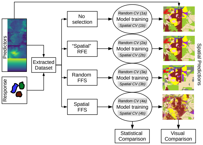
The load-bearing mechanism is forward feature selection (FFS) driven by spatial cross-validation. FFS starts from the two-predictor model with the best spatial validation score, then adds predictors one at a time only if they improve that score; variables that do not help spatial prediction are excluded. Because the cross-validation folds are spatial blocks or held-out clusters, a variable that only memorizes training-location patterns cannot earn a place in the model. This contrasts with Random Forest's internal out-of-bag importance and with recursive feature elimination, which rank variables by how well they fit the training data and therefore keep the very geolocation variables that cause spatial overfitting.

What would settle it

On a spatially clustered dataset with coordinates and elevation as candidate predictors, train Random Forest with and without spatial forward feature selection and compare spatial block-CV predictions; if the full model shows no linear map artefacts and no worse spatial CV error than the spectrally selected model, the central claim that geolocation predictors cause spatial overfitting would fail.

Watch

Extended reading notes

Core claim

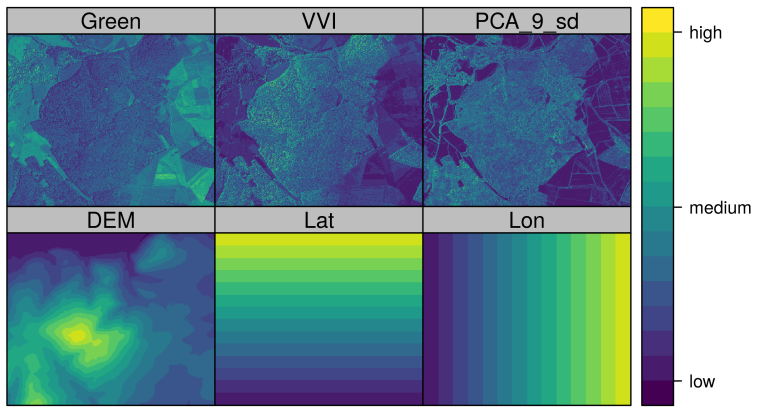
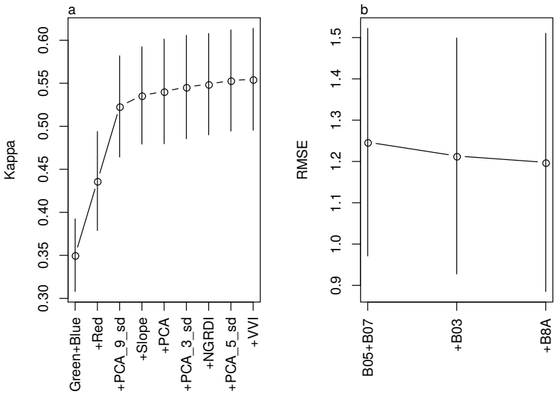
The central discovery is that Random Forest models trained on spatially clustered field data treat highly autocorrelated geolocation variables (latitude, longitude, elevation) as if they carried environmental signal, when in fact they encode the locations of the training clusters. The result is a model that scores above 0.99 Kappa or an R-squared near 0.87 under random cross-validation but drops to 0.55 Kappa or an R-squared of 0.58 under spatial block cross-validation, and it produces maps with linear boundaries that do not match the underlying imagery. Recursive feature elimination does not fix this, because those misleading variables rank as the most important according to the algorithm's training-based importance measure. Forward feature selection evaluated with spatial cross-validation automatically drops the geolocation variables, leaves only spectral predictors (plus slope for land cover), removes the linear artefacts, and slightly raises spatial validation performance (Kappa 0.56; global R-squared 0.63 for leaf area index). The paper concludes that spatial validation alone is insufficient: the variable selection step itself must use spatial cross-validation.

Load-bearing premise

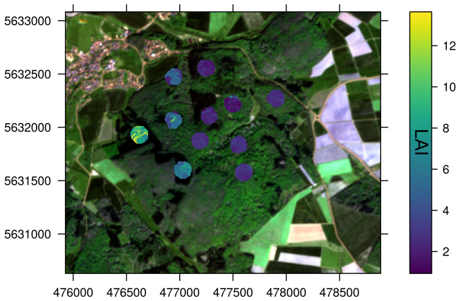
The leaf-area-index demonstration assumes that lidar-derived leaf area index from 2010 is a valid reference for predictions built on 2017 Sentinel-2 imagery, because no major forest management occurred in between; if the canopy changed during those seven years, the regression labels would be partly wrong and the comparison of variable-selection strategies would be unreliable.

Editorial extensions

If this is right

Spatial cross-validation should be part of every step of spatial machine-learning modelling, including predictor selection and hyperparameter tuning, not just final validation.
Recursive feature elimination, common in environmental mapping, will not remove geographically misleading predictors because it ranks variables by training importance.
Including coordinates or other location-derived fields as predictors in spatially clustered designs risks producing maps with artificial linear boundaries, even when overall accuracy statistics look acceptable under random validation.
Statistical spatial performance alone cannot distinguish a reliable spatial model from one with artefacts; visual inspection of prediction maps is needed in practice.
Spatial FFS changed the prediction maps considerably even where statistical performance changed only slightly, so quantitative metrics alone would miss the improvement.

Reading between the lines

Editorial extensions of the paper, not claims the author makes directly.

The failure mode identified here should generalize to any flexible learner, not just Random Forests, whenever training samples are spatially clustered and predictors include smoothly varying location fields.
The benefit of spatial variable selection is likely to scale with the strength of spatial autocorrelation and the degree of clustering; on near-random sampling designs, the gap between random and spatial FFS should shrink, a prediction that could be tested by simulation.
Linear map artefacts caused by geolocation predictors could be turned into an automated diagnostic: scanning prediction maps for axis-aligned discontinuities as a cheap screen for spatial overfitting.
The same spatial-selection logic applies to temporal or spatio-temporal prediction, where date or time-index variables could play the role of latitude and longitude.

Share X Bluesky LinkedIn Reddit HN

Signed reviews

No signed human review yet.

Editorial analysis

A structured set of objections, weighed in public.

Desk editor's note, referee report, and a circularity audit.

Desk Editor's Note

read the letter

Colleague,

You should know about arXiv:1908.07805 if you work on spatial prediction with machine learning. It gives a clean, reproducible demonstration that including coordinates and elevation as predictors leads to visible artifacts in Random Forest maps, and that a forward feature selection run with spatial cross-validation drops those predictors and cleans up the maps. The paper is a follow-up to the authors' own FFS paper (Meyer et al. 2018), so it is not a new method. The new material is two case studies (LULC classification and LAI regression) plus a comparison against RFE and random FFS. That comparison is the real value: RFE, even with spatial CV, does not remove latitude/longitude because they rank highly in variable importance; random FFS makes the artifacts worse. These are useful negative controls, and the visual evidence is striking. Code and data links are included.

Where I part company with the abstract is the quantitative claim. Models 4a/4b are built by running FFS inside spatial CV and then evaluated on the same spatial CV folds. That is double use of the test folds. The reported improvements (Kappa 0.55 to 0.56, RMSE 1.25 to 1.20, R2 0.58 to 0.63) are selection-biased and should not be read as unbiased estimates of spatial predictive performance. The paper needs an outer/inner nested resampling scheme (outer spatial CV for evaluation, inner spatial CV for FFS) before claiming improved statistical spatial model performance. The visual argument is independent and survives, but the headline statistical gain is not established.

The LAI case study has a second, smaller caveat: lidar reference data from 2010 are paired with Sentinel-2 predictors from 2017. The authors disclose this and argue the forest was stable; that is plausible but it makes the LAI comparison a bit fragile. If the canopy changed in those seven years, the labels are noisy and the variable-selection comparison for the regression task is weakened.

Overall this is a serious, readable paper that makes a practical point: spatial validation alone does not fix a model that is overfitting to geolocation variables; you need spatial feature selection too. The demonstration is convincing visually, and the negative controls are good. The statistical support needs repair, and the novelty is incremental. But it deserves a serious referee. I would send it to review with a request for nested spatial CV, confidence intervals on the performance differences, and a more cautious wording of the abstract.

Best

Referee Report

3 major / 4 minor

Summary. The paper argues that standard machine learning practice for spatial prediction, which typically ignores spatial autocorrelation during model building, produces models that reproduce training data but fail when predicting beyond training locations. The authors use two case studies (land use/land cover classification and leaf area index regression) with Random Forests to compare random versus spatial cross-validation and several variable selection strategies, including recursive feature elimination, forward feature selection with random CV, and forward feature selection with spatial CV. They report that spatial CV strongly lowers estimated performance compared to random CV, that geolocation predictors such as latitude and longitude dominate variable importance and create visible artefacts in prediction maps, and that spatial forward feature selection removes these predictors and yields qualitatively more plausible maps with slightly better spatial CV statistics.

Significance. If the central claim is supported, the paper makes a useful methodological contribution: it demonstrates that spatial variable selection, not only spatial validation, should be part of spatial machine learning pipelines. The study is well positioned in the recent literature on spatial CV and benefits from two independent case studies, a negative control (random FFS and RFE) that performs worse, and publicly available code on GitHub. The visual artefact evidence from geolocation predictors is compelling and should be reproducible by readers. However, the quantitative support for the central claim is weakened by a selection-bias issue in the evaluation of the spatial FFS models and by a temporal mismatch in the LAI reference data, as detailed below.

major comments (3)

[Section 2.3.2 and Tables 2-3, models 4a/4b] The spatial performance of the spatial-FFS models is not an unbiased estimate because the same spatial CV folds are used both to select the variables and to evaluate the final model. In Section 2.3.2, FFS with spatial CV uses all folds to choose the variable subset; the subsequent re-training and spatial CV evaluation of models 4a/4b then tests on folds that already influenced the variable selection. This is a classic selection-bias error. The reported gains from spatial FFS are small (Kappa 0.55 to 0.56; RMSE 1.25 to 1.20; global R2 0.58 to 0.63) and are not accompanied by significance tests or confidence intervals, so they cannot support the abstract's claim of 'improved statistical spatial model performance.' Please re-run the analysis with nested spatial CV (outer folds for evaluation, inner folds for FFS), or, if the visual pattern assessment is the primary evidence, state that explicitly and temper the statistical claim accordingly.
[Section 2.2.1 and Table 3] The LAI reference data are from lidar acquired in 2010, while the Sentinel-2 predictors are from May 2017. The authors justify this by stating that no major management occurred, but natural forest growth, phenology, and small-scale disturbance over seven years can change LAI and canopy structure. If the lidar-derived LAI does not represent the forest state at the time of the Sentinel-2 image, the training labels are incorrect, making the reported RMSE and R2 values in Table 3 and the LAI-based conclusions in Sections 3.3 and 4.2 unreliable. Please either use temporally matching reference data, restrict the LAI case study to a sensitivity analysis, or clearly frame the LAI results as illustrative with this caveat prominently stated.
[Section 4.3 and Abstract] The discussion states that the model using all predictors and the model using spatially selected variables 'perform equally well, statistically speaking' under spatial CV, while the abstract claims that spatial variable selection leads to 'improved statistical spatial model performance.' Given the small and untested differences in Tables 2 and 3, these two statements are in tension. The quantitative claim should be based on nested CV estimates (or equivalent unbiased evaluation) or explicitly downgraded to a qualitative/visual claim, so that the paper's conclusion is internally consistent.

minor comments (4)

[Figure 4 and Section 2.3] The acronyms 'CV', 'FFS', and 'RFE' are used in Figure 4 before they are defined in the text; please define them in the figure caption or introduce them before the figure.
[Figure 6] The colors used to indicate the 11 folds are not easily distinguishable in grayscale or for color-deficient readers; please use a colorblind-safe palette or add direct labels to the points.
[Table 3] The per-fold R2 values for spatial CV are near zero for all models, and although the text explains this as a consequence of low within-fold variability, the table itself is misleading without that caveat; consider reporting only global R2 or adding a footnote to the table.
[References] Several references are preprints or non-peer-reviewed versions (e.g., Valavi et al. 2018 bioRxiv, Hengl et al. 2018 preprint); please update to the published versions where available.

Circularity Check

1 steps flagged · score 6.0 of 10

Spatial-FFS performance is evaluated on the same CV folds used for variable selection, so the reported statistical gains are selection-biased; the visual artifact evidence remains independent.

fitted input called prediction [Section 2.3.2 (Spatial predictor variable selection) and Table 3, model 4b]
"This FFS implementation works in conjunction with user-defined cross-validation, hence it allows to select variables that lead to the highest spatial performance (if run in conjunction with spatial CV). First, the FFS trains models using every combination of two-predictor variables. Based on the best performing variables (as identified by cross-validation), FFS increases the number of variables to test which (if any) variables further improve the (spatial) models performance. ..."

FFS is a greedy optimization of the variable set against spatial-CV performance computed on the full dataset. Model 4b then reports the spatial-CV performance of a model trained with the selected variables using the same spatial-CV fold partition. No outer/nested CV is used, so the left-out spatial folds have already influenced the choice of variables through the selection criterion. Consequently the reported Kappa=0.56, RMSE=1.20, and R2=0.63 are selection-criterion optima rather than predictions for unseen locations, and the tiny gains over the full model (Kappa 0.55, RMSE 1.25, R2 0.58) are within the bias created by reusing the folds.

full rationale

The paper's visual artifact demonstration is not circular: the full model and the random-FFS model produce clear linear artifacts that are traced to geolocation predictors, and the spatial-FFS model produces spectrally driven predictions without such artifacts. Those observations are empirical and independent of any fitted parameter. Self-citations to Meyer et al. (2018) and the CAST package are present, but they supply the FFS algorithm rather than the evidence, and the code is provided, so they are not load-bearing in a circular sense. The LAI reference-time-lag issue is a data-quality concern, not circularity. The central circularity is the double use of the same spatial CV folds for variable selection and for reporting the spatial performance of the selected-variable model (model 4b). Because the variables were chosen to maximize spatial-CV performance on those folds, the reported statistical improvement is a selection-biased re-statement of the selection criterion rather than an unbiased prediction for new spatial locations. This affects the quantitative conclusion but not the independent visual evidence, so the analysis is partially circular rather than wholly reducible to its inputs.

Assumptions & free parameters 0 free parameters · 4 assumptions · 0 invented entities

The paper is an empirical case study, not a derivation. It does not fit free parameters beyond standard hyperparameters like mtry and tree count, which are tuned and not load-bearing. The key assumptions are about data validity: the 2010 lidar LAI as ground truth for 2017 imagery, the adequacy of spatial blocking CV, and the correctness of manually digitized labels.

assumptions (4)

domain assumption Random Forest with 500 trees and tuned mtry is an adequate model for LULC classification and LAI regression.
The paper selects this algorithm because of its prominence, without formal justification of its suitability for these specific tasks.
domain assumption Spatial block and leave-one-cluster-out cross-validation provide valid estimates of predictive performance beyond the training locations.
The paper assumes these hold-out strategies are a good proxy for real spatial generalization.
ad hoc to paper The lidar-derived LAI reference from 2010 represents the forest state at the time of the 2017 Sentinel-2 image.
Explicitly assumed in Section 2.2.1 despite a seven-year gap; the authors state no major management occurred.
domain assumption Manually digitized LULC polygons are an accurate reference for the classification task.
Reference data were created by visual inspection and field knowledge, which is standard but not independently verified.

how reviews work

0 comments

Cite this review

Pith. "Pith review of Importance of spatial predictor variable selection in machine learning applications -- Moving from data reproduction to spatial prediction." pith.science (2026). https://pith.science/paper/CTX23BB3

@misc{pith2026190807805,
  author       = {Pith},
  title        = {Pith review of: Importance of spatial predictor variable selection in machine learning applications -- Moving from data reproduction to spatial prediction},
  year         = {2026},
  howpublished = {\url{https://pith.science/paper/CTX23BB3}},
  note         = {Machine review of arXiv:1908.07805}
}

read the original abstract

Machine learning algorithms find frequent application in spatial prediction of biotic and abiotic environmental variables. However, the characteristics of spatial data, especially spatial autocorrelation, are widely ignored. We hypothesize that this is problematic and results in models that can reproduce training data but are unable to make spatial predictions beyond the locations of the training samples. We assume that not only spatial validation strategies but also spatial variable selection is essential for reliable spatial predictions. We introduce two case studies that use remote sensing to predict land cover and the leaf area index for the "Marburg Open Forest", an open research and education site of Marburg University, Germany. We use the machine learning algorithm Random Forests to train models using non-spatial and spatial cross-validation strategies to understand how spatial variable selection affects the predictions. Our findings confirm that spatial cross-validation is essential in preventing overoptimistic model performance. We further show that highly autocorrelated predictors (such as geolocation variables, e.g. latitude, longitude) can lead to considerable overfitting and result in models that can reproduce the training data but fail in making spatial predictions. The problem becomes apparent in the visual assessment of the spatial predictions that show clear artefacts that can be traced back to a misinterpretation of the spatially autocorrelated predictors by the algorithm. Spatial variable selection could automatically detect and remove such variables that lead to overfitting, resulting in reliable spatial prediction patterns and improved statistical spatial model performance. We conclude that in addition to spatial validation, a spatial variable selection must be considered in spatial predictions of ecological data to produce reliable predictions.

Figures

Figures reproduced from arXiv: 1908.07805 by the authors.

**Figure 2.** Example of spectral, terrain-related and geolocation predictor variables: re [PITH_FULL_IMAGE:figures/full_fig_p007_2.png] view at source ↗

**Figure 3.** Study area represented by the true color composite of the Sentinel-2 scene, [PITH_FULL_IMAGE:figures/full_fig_p009_3.png] view at source ↗

Figures from the paper (7 more)

**Figure 4.** Figure 4: Overview on the models compared in this study. Spectral, terrain related as [PITH_FULL_IMAGE:figures/full_fig_p012_4.png]

**Figure 5.** Figure 5: Concept of random and spatial cross-validation (CV): A total dataset (here: [PITH_FULL_IMAGE:figures/full_fig_p014_5.png]

**Figure 6.** Figure 6: Comparison between observed and predicted LAI values based on random (a) [PITH_FULL_IMAGE:figures/full_fig_p018_6.png]

**Figure 7.** Figure 7: Relative scaled importance of the predictor variables within the Random Forest [PITH_FULL_IMAGE:figures/full_fig_p020_7.png]

**Figure 8.** Figure 8: Performance of FFS with variables selected by spatial cross-validation for pre [PITH_FULL_IMAGE:figures/full_fig_p021_8.png]

**Figure 9.** Figure 9: RGB representation of the study area on the basis of the aerial image (RGB), [PITH_FULL_IMAGE:figures/full_fig_p022_9.png]

**Figure 10.** Figure 10: RGB representation of the study area on the basis of the Sentinel-2 image [PITH_FULL_IMAGE:figures/full_fig_p023_10.png]

Discussion (0). Continue with ORCID to comment.

Reference graph

Works this paper leans on

13 extracted references · 11 canonical work pages

[1]

R., Hemp, A., & Nauss, T

Appelhans, T., Mwangomo, E., Hardy, D. R., Hemp, A., & Nauss, T. (2015). Evaluating machine learning approaches for the interpolation of monthly air temperature at Mt. Kilimanjaro, Tanzania. Spatial Statistics, 14, Part A, 91–113. URL: https://doi.org/10.1016/j.spasta.2015.05.008. Attorre, F., Alf, M., Sanctis, M. D., Francesconi, F., Valenti, R., Vitale,...

work page arXiv 2015
[9]

org/10.1016/j.envsoft.2017.12.001

URL: https://doi. org/10.1016/j.envsoft.2017.12.001. doi:https://doi.org/10.1016/ j.envsoft.2017.12.001. Micheletti, N., Foresti, L., Robert, S., Leuenberger, M., Pedrazzini, A., Jaboyedoﬀ, M., & Kanevski, M. (2014). Machine Learning Feature Se- lection Methods for Landslide Susceptibility Mapping. Math. Geosci., 46 , 33–57. Planetary Habitability Laborat...

arXiv 2014
[11]

28 com/science/article/pii/S0098300416303909

URL: http://www.sciencedirect. 28 com/science/article/pii/S0098300416303909. doi:https://doi.org/ 10.1016/j.cageo.2017.02.012. Cohen, J. (1960). A coeﬃcient of agreement for nominal scales. Educa- tional and Psychological Measurement , 20 , 37–46. URL: https://doi. org/10.1177/001316446002000104. doi: 10.1177/001316446002000104. arXiv:https://doi.org/10.1...

work page arXiv 1960
[112]

com/science/article/pii/S0303243412001791

URL: http://www.sciencedirect. com/science/article/pii/S0303243412001791. doi:https://doi.org/ 10.1016/j.jag.2012.07.020. Janatian, N., Sadeghi, M., Sanaeinejad, S. H., Bakhshian, E., Farid, A., Hasheminia, S. M., & Ghazanfari, S. (2017). A statistical framework for estimating air temperature using MODIS land surface temperature data. Int. J. Climatol. , ...

work page doi:10.1016/j.jag.2012.07.020 2017
[114]

doi: https://doi.org/10.1016/j.jag.2015

URL: http://www.sciencedirect.com/science/article/ pii/S0303243415001178. doi: https://doi.org/10.1016/j.jag.2015. 05.008. Kuhn, M. (2016). caret: Classiﬁcation and Regression Training . URL: https://CRAN.R-project.org/package=caret R package version 6.0-68. Kuhn, M., & Johnson, K. (2013). Applied Predictive Modeling . (1st ed.). New York: Springer. Lange...

work page doi:10.1016/j.jag.2015 2016
[120]

doi:https://doi.org/10.1016/j.ecolmodel

URL: http://www.sciencedirect.com/science/article/ pii/S0304380019302145. doi:https://doi.org/10.1016/j.ecolmodel. 2019.06.002. Shi, Y., Song, L., Xia, Z., Lin, Y., Myneni, R. B., Choi, S., Wang, L., Ni, X., Lao, C., & Yang, F. (2015). Mapping Annual Precipitation across Mainland China in the Period 2001-2010 from TRMM3B43 Product Us- ing Spatial Downscal...

work page doi:10.1016/j.ecolmodel 2015
[246]

1007/s10661-016-5238-y

URL: https://doi.org/10. 1007/s10661-016-5238-y . doi:10.1007/s10661-016-5238-y . Schratz, P., Muenchow, J., Iturritxa, E., Richter, J., & Brenning, A. (2019). Hyperparameter tuning and performance assessment of statistical and machine-learning algorithms using spatial data. Ecological Modelling, 406 , 109 –

work page doi:10.1007/s10661-016-5238-y 2019
[732]

Meyer, H., K¨ uhnlein, M., Reudenbach, C., & Nauss, T

URL: https://doi.org/ 10.3390/rs8090732. Meyer, H., K¨ uhnlein, M., Reudenbach, C., & Nauss, T. (2017a). Reveal- ing the potential of spectral and textural predictor variables in a neural network-based rainfall retrieval technique. Remote Sensing Letters , 8 , 647–656. URL: https://doi.org/10.1080/2150704X.2017.1312026. Meyer, H., Lehnert, L. W., Wang, Y....

work page arXiv 2017

Show all 13 references

[820]

doi: 10.1111/geb

URL: http://dx.doi.org/10.1111/geb.12161. doi: 10.1111/geb. 12161. Li, J., Heap, A. D., Potter, A., & Daniell, J. J. (2011). Application of ma- chine learning methods to spatial interpolation of environmental variables. Environmental Modelling & Software , 26 , 1647–1659. Liaw...

2011 doi
[835]

Juel, A., Groom, G

URL: https: //doi.org/10.3390/rs8100835. Juel, A., Groom, G. B., Svenning, J.-C., & Ejrns, R. (2015). Spatial application of Random Forest models for ﬁne-scale coastal vegetation classiﬁcation using object based analysis of aerial or- thophoto and DEM data. Int. J. Appl. Earth...

2015 doi
[2879]

Hengl, T., Nussbaum, M., Wright, M., Heuvelink, G., & Grler, B. (2018). Random forest as a generic framework for predictive modeling of spatial and spatio-temporal variables. PeerJ Preprints , . doi: 10.7287/peerj. preprints.26693v3. Hessische Verwaltung f¨ ur Bodenmanagement ...

2018 doi
[4766]

Jing, W., Yang, Y., Yue, X., & Zhao, X. (2016). A Comparison of Dif- ferent Regression Algorithms for Downscaling Monthly Satellite-Based Precipitation over North China. Remote Sensing , 8 ,

2016
[6940]

Wenger, S

URL: https: //doi.org/10.1038/s41598-017-07197-6 . Wenger, S. J., & Olden, J. D. (2012). Assessing transferability of ecological models: an underappreciated aspect of statistical val- idation. Methods in Ecology and Evolution , 3 , 260–267. URL: https://besjournals.onlinelibra...

2012 arXiv

Pith tools

Reviewed August 14, 2026 · model on record in the stance chip above.

[1] [1]

R., Hemp, A., & Nauss, T

Appelhans, T., Mwangomo, E., Hardy, D. R., Hemp, A., & Nauss, T. (2015). Evaluating machine learning approaches for the interpolation of monthly air temperature at Mt. Kilimanjaro, Tanzania. Spatial Statistics, 14, Part A, 91–113. URL: https://doi.org/10.1016/j.spasta.2015.05.008. Attorre, F., Alf, M., Sanctis, M. D., Francesconi, F., Valenti, R., Vitale,...

work page arXiv 2015

[2] [9]

org/10.1016/j.envsoft.2017.12.001

URL: https://doi. org/10.1016/j.envsoft.2017.12.001. doi:https://doi.org/10.1016/ j.envsoft.2017.12.001. Micheletti, N., Foresti, L., Robert, S., Leuenberger, M., Pedrazzini, A., Jaboyedoﬀ, M., & Kanevski, M. (2014). Machine Learning Feature Se- lection Methods for Landslide Susceptibility Mapping. Math. Geosci., 46 , 33–57. Planetary Habitability Laborat...

arXiv 2014

[3] [11]

28 com/science/article/pii/S0098300416303909

URL: http://www.sciencedirect. 28 com/science/article/pii/S0098300416303909. doi:https://doi.org/ 10.1016/j.cageo.2017.02.012. Cohen, J. (1960). A coeﬃcient of agreement for nominal scales. Educa- tional and Psychological Measurement , 20 , 37–46. URL: https://doi. org/10.1177/001316446002000104. doi: 10.1177/001316446002000104. arXiv:https://doi.org/10.1...

work page arXiv 1960

[4] [112]

com/science/article/pii/S0303243412001791

URL: http://www.sciencedirect. com/science/article/pii/S0303243412001791. doi:https://doi.org/ 10.1016/j.jag.2012.07.020. Janatian, N., Sadeghi, M., Sanaeinejad, S. H., Bakhshian, E., Farid, A., Hasheminia, S. M., & Ghazanfari, S. (2017). A statistical framework for estimating air temperature using MODIS land surface temperature data. Int. J. Climatol. , ...

work page doi:10.1016/j.jag.2012.07.020 2017

[5] [114]

doi: https://doi.org/10.1016/j.jag.2015

URL: http://www.sciencedirect.com/science/article/ pii/S0303243415001178. doi: https://doi.org/10.1016/j.jag.2015. 05.008. Kuhn, M. (2016). caret: Classiﬁcation and Regression Training . URL: https://CRAN.R-project.org/package=caret R package version 6.0-68. Kuhn, M., & Johnson, K. (2013). Applied Predictive Modeling . (1st ed.). New York: Springer. Lange...

work page doi:10.1016/j.jag.2015 2016

[6] [120]

doi:https://doi.org/10.1016/j.ecolmodel

URL: http://www.sciencedirect.com/science/article/ pii/S0304380019302145. doi:https://doi.org/10.1016/j.ecolmodel. 2019.06.002. Shi, Y., Song, L., Xia, Z., Lin, Y., Myneni, R. B., Choi, S., Wang, L., Ni, X., Lao, C., & Yang, F. (2015). Mapping Annual Precipitation across Mainland China in the Period 2001-2010 from TRMM3B43 Product Us- ing Spatial Downscal...

work page doi:10.1016/j.ecolmodel 2015

[7] [246]

1007/s10661-016-5238-y

URL: https://doi.org/10. 1007/s10661-016-5238-y . doi:10.1007/s10661-016-5238-y . Schratz, P., Muenchow, J., Iturritxa, E., Richter, J., & Brenning, A. (2019). Hyperparameter tuning and performance assessment of statistical and machine-learning algorithms using spatial data. Ecological Modelling, 406 , 109 –

work page doi:10.1007/s10661-016-5238-y 2019

[8] [732]

Meyer, H., K¨ uhnlein, M., Reudenbach, C., & Nauss, T

URL: https://doi.org/ 10.3390/rs8090732. Meyer, H., K¨ uhnlein, M., Reudenbach, C., & Nauss, T. (2017a). Reveal- ing the potential of spectral and textural predictor variables in a neural network-based rainfall retrieval technique. Remote Sensing Letters , 8 , 647–656. URL: https://doi.org/10.1080/2150704X.2017.1312026. Meyer, H., Lehnert, L. W., Wang, Y....

work page arXiv 2017