REVIEW 3 major objections 5 minor 45 references
Semi-supervised Sequence Modeling for Elastic Impedance Inversion
T0 review · 3 major / 5 minor · reviewed 2026-08-14 · deepseek-v4-flash
Pith's one-line read Semi-supervised networks invert elastic impedance to 98% correlation with only 10 training wells.
desk verdict A solid, clearly presented semi-supervised inversion method whose headline 98% is a self-consistency result on the same forward model used for generation and constraint, so read the real-data claim cautiously. read the letter →
The pith
A machine-rendered reading of the paper's core claim, the machinery that carries it, and where it could break.
The reading
What carries the argument
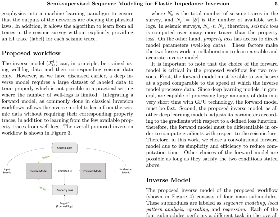
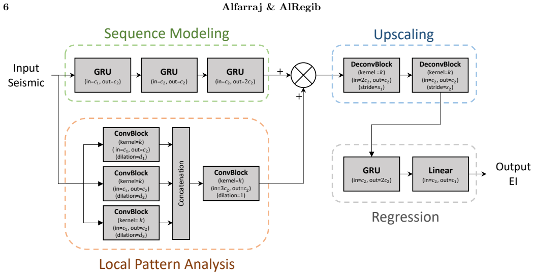
The central mechanism is a differentiable loop in which a forward model checks the geophysical plausibility of the network's output at every seismic trace. The forward model computes angle-dependent reflection coefficients from estimated EI as $RC(t,\theta)=\frac{1}{2}\frac{EI(t+\Delta t,\theta)-EI(t,\theta)}{EI(t+\Delta t,\theta)+EI(t,\theta)}$ and synthesizes a seismogram by convolution with a wavelet; the inverse model is a bidirectional GRU stack for the low-frequency EI trend plus parallel dilated convolutions for high-frequency local detail, followed by deconvolutional upscaling and a final regression GRU. The training objective is the sum of a property loss on labeled well traces and a seismic loss on all traces, so every unlabeled trace contributes a physics-based constraint.
What would settle it
Run the trained inversion on a real survey with well-log EI measurements held out, using a wavelet and velocity model estimated independently of the training data; if average PCC on the held-out wells falls well below the synthetic 98% while the seismic loss stays low, or if perturbing the assumed wavelet materially changes the inverted EI, the central claim of forward-model-regularized semi-supervised inversion is not supported for field use.
Extended reading notes
Core claim
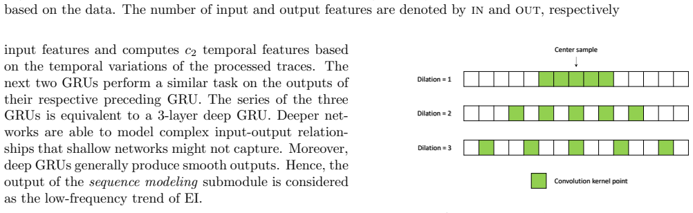
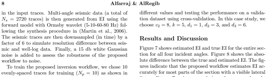
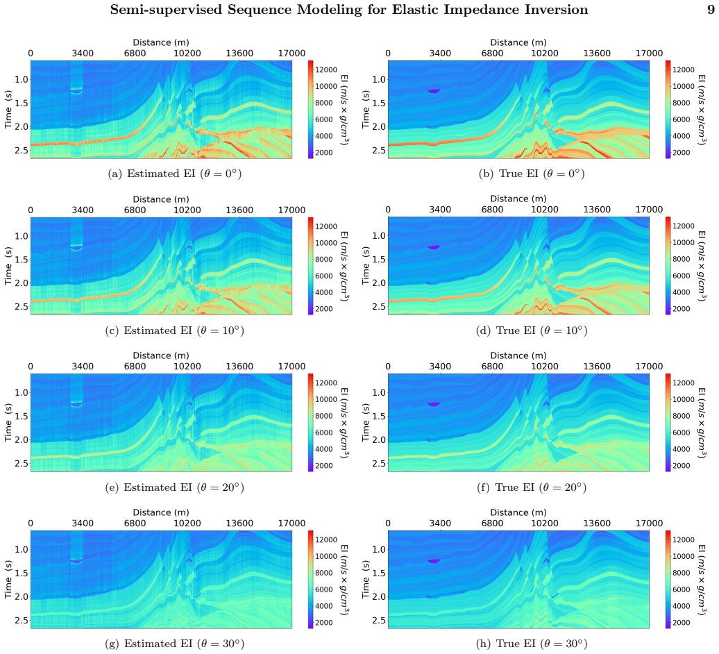
On its own terms, the paper establishes that a semi-supervised sequence-modeling inversion network can recover elastic impedance from multi-angle seismic data almost exactly with very few labels. The inverse model combines a deep bidirectional GRU stack, which supplies the low-frequency trend of EI, with parallel dilated convolutional blocks, which supply high-frequency local detail; deconvolution layers upscale to well-log resolution, and a final GRU plus linear layer regresses to EI. The training objective is the sum of a property loss on the 10 labeled traces and a seismic loss, computed by passing the estimated EI through the elastic-impedance reflection-coefficient formula and convolving with a wavelet, then comparing to the input seismic traces across all 2720 traces. With both losses active, average PCC is 0.98, $r^2$ is 0.94, and M-SSIM is 0.92; supervision alone reaches 0.96/0.88/0.87, while the seismic loss alone collapses to 0.33/-0.45/0.77.
Load-bearing premise
The load-bearing premise is that the convolutional forward model (elastic-impedance reflection coefficients convolved with a wavelet) accurately represents real seismic data generation, and the synthetic validation uses that same model to create the data, so it does not test the premise against real-field mismatch.
Editorial extensions
If this is right
- The seismic-loss term lets the network use every seismic trace in a survey, so the labeled-well requirement can drop to a handful of traces.
- The same workflow should extend to full elastic inversion or other rock-property estimation by changing the target variable and the forward model.
- The comparison in Table 2 implies that purely data-driven unsupervised inversion is unreliable here (PCC 0.33), so forward-model regularization is what makes the 98% result possible.
- Inversion runs in about two minutes on one GPU for 500 iterations, suggesting the method is practical for survey-scale use, with computation scaling linearly in the number of traces.
Reading between the lines
- Because the synthetic seismic data are generated with the same forward model used as the seismic loss, the 98% figure likely overstates what mismatched real-field data would deliver; the paper does not include a field-data test.
- The visible lateral jitter between neighboring traces suggests that adding a spatial or structural constraint to the 1D sequence model could further improve section quality without changing the training scheme.
- The method's dependence on a differentiable forward model invites a natural extension: train with an ensemble of plausible wavelets or a parameterized wavelet so the inversion becomes robust to wavelet uncertainty.
- Since EI reduces to acoustic impedance at zero offset, the same architecture with a single input channel should perform acoustic impedance inversion; a positive result there would indicate the mechanism is generic to impedance-type inversion.
Signed reviews
Editorial analysis
A structured set of objections, weighed in public.
Referee Report
Summary. The paper proposes a semi-supervised sequence-modeling framework, based on bidirectional GRUs and convolutional layers, to invert multi-angle seismic data for elastic impedance (EI). The training loss combines a supervised term on well-log traces (property loss) with a seismic data-misfit term computed by passing the estimated EI through a differentiable convolutional forward model (seismic loss). The method is validated on the Marmousi 2 synthetic model using 10 evenly spaced well logs, reporting an average Pearson correlation of 0.98, an average r² of 0.94, and M-SSIM of 0.92, with an ablation showing that the semi-supervised scheme outperforms both supervised-only and unsupervised-only variants.
Significance. If the results hold under realistic conditions, the contribution is valuable: embedding a differentiable forward model directly into a deep-learning loss is a principled way to incorporate geophysical constraints and reduce dependence on scarce well labels. The paper is clearly written, the methodology is well structured, and the authors make code publicly available, which strengthens reproducibility. However, the headline accuracy is demonstrated only in a self-consistent setting where the forward model used inside the loss is identical to the model that generated the synthetic data. This leaves the practical significance of the 'geophysical constraint' claim uncertain, because forward-model misspecification is a central risk in real-data applications.
major comments (3)
- [Forward Model and Dataset Generation (Eqs. 10–12)] The seismic loss L2 in Eq. (9) uses exactly the same convolutional forward model described by Eqs. (10)–(12) that was used to generate the synthetic seismic data in the Dataset Generation section. Consequently, the reported 0.98 PCC in Table 1 is in part a cycle-consistency result under a known generator, and the validation does not test the method under forward-model misspecification. This is load-bearing for the paper's central claim that the seismic loss acts as a meaningful geophysical constraint, especially since the paper itself states that 'the choice of the forward model is critical in the proposed workflow.' I recommend adding a robustness experiment with an independent or perturbed forward model (e.g., a different wavelet, full Zoeppritz instead of the Aki–Richards/EI approximation, or a systematically biased velocity ratio) and reporting whether the inversion degrades gracefully.
- [Case Study on Marmousi 2 Model, Dataset Generation and Table 1] The quantitative results in Table 1 are based on a single realization: one noise draw, one choice of 10 evenly spaced training wells, and one hyperparameter configuration. Because well placement strongly affects semi-supervised learning, and because the evenly spaced wells constitute a favorable sampling that may not occur in practice, the reported PCC and r² values need accompanying variance estimates. Please report multiple runs with different random well selections and noise realizations, and discuss the regular spacing as a favorable condition rather than a general setting.
- [Results and Discussion, Table 2] The ablation in Table 2 compares supervised (α=1, β=0) and semi-supervised (α=1, β=1) training, but the semi-supervised model additionally uses all unlabeled traces through the seismic loss while the supervised model uses only 10 labeled traces. This is a reasonable high-level comparison, but it does not isolate the contribution of the physical forward model from the general benefit of having more training data. A more controlled comparison—for example, replacing L2 with a non-physical smoothness regularizer, or computing L2 with a deliberately misspecified forward model—would directly test whether the geophysical constraint, rather than merely the additional data, is responsible for the improvement.
minor comments (5)
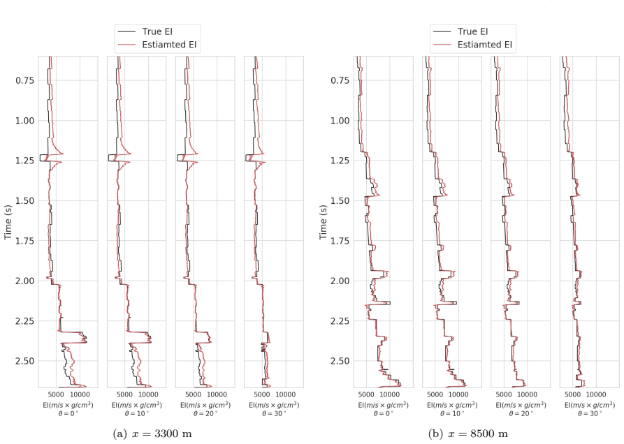
- [Results and Discussion, Figure 9] The text refers to the selected trace at x = 3200 m, but the caption of Figure 9 labels it as x = 3300 m; please correct the inconsistency.
- [Methodology, Eq. (9)] The loss in Eq. (9) divides the property loss by Np and the seismic loss by Ns, while the implementation section states that traces are normalized before training; please clarify how the normalization interacts with the weighting α=β=1, since the two terms have very different numbers of samples.
- [Case Study, Hyperparameters] The hyperparameters c2=8, k=5, d1=1, d2=3, d3=6 are stated, but no sensitivity analysis or validation-split details are provided; adding this information would improve reproducibility and help readers transfer the method to other datasets.
- [Results and Discussion, Eq. (15)] The SSIM formula uses α, β, γ as tunable constants, but the parameter values used to compute M-SSIM are not reported; please state them and confirm whether the standard SSIM setting (α=β=γ=1) is used.
- [Forward Model, Eq. (10)] The reflection coefficient in Eq. (10) is written as a function of EI at t and t+Δt; please specify the time grid and the relationship between the vertical sampling of the seismic data and the EI traces, since this affects the convolutional forward model and the upscaling module.
Circularity Check
No significant circularity: the 98% result is evaluated against an independently defined Marmousi EI target; sharing the forward model between data generation and seismic loss is a validation limitation, not a circular reduction.
full rationale
The derivation chain is not circular. The target EI traces are generated from the Marmousi 2 elastic model via the Whitcombe/Connolly formula, so the labels used in the property loss L1 are independent of the network and of any fitted parameter. The seismic loss L2 does use the same convolutional forward model (Eqs. 10–12) that generated the synthetic seismic data, which makes the synthetic test a self-consistency check under a known generator and leaves forward-model misspecification unexplored; but this does not make the predicted EI a relabeled fitted quantity. The network is not initialized with the target, and the 98% correlation is not forced by construction: it requires the learned inverse mapping to reproduce unseen EI traces, anchored by only 10 well-log traces. The self-citations to the authors' prior RNN work are motivational and are not load-bearing; no uniqueness theorem or unverified prior result is imported to forbid alternatives. The only substantive concern is external validity under a mismatched forward model, which the paper itself flags ('the choice of the forward model is critical in the proposed workflow'), and that is a correctness/robustness caveat rather than a circularity. No step meets the required bar of a predicted quantity being equivalent to its input by definition or by a fitted-parameter renaming.
Assumptions & free parameters
free parameters (2)
- Network hyperparameters (c2, k, d1, d2, d3, s1, s2) =
c2=8, k=5, d1=1, d2=3, d3=6, s1=3, s2=2
- Loss weighting coefficients (alpha, beta) =
alpha=1, beta=1
assumptions (4)
- domain assumption The convolutional forward model (Eqs. 10-12) accurately represents the seismic response of the subsurface.
- domain assumption The Aki-Richards approximation and normalized elastic impedance (Eq. 11) are valid for the incident angles used (0 to 30 degrees).
- domain assumption The Marmousi 2 model is a representative testbed for evaluating inversion performance.
- standard math Backpropagation through the differentiable forward model yields useful gradients for the seismic loss.
Cite this review
Pith. "Pith review of Semi-supervised Sequence Modeling for Elastic Impedance Inversion." pith.science (2026). https://pith.science/paper/36ZS22D5
@misc{pith2026190807849,
  author       = {Pith},
  title        = {Pith review of: Semi-supervised Sequence Modeling for Elastic Impedance Inversion},
  year         = {2026},
  howpublished = {\url{https://pith.science/paper/36ZS22D5}},
  note         = {Machine review of arXiv:1908.07849}
}
read the original abstract
Recent applications of machine learning algorithms in the seismic domain have shown great potential in different areas such as seismic inversion and interpretation. However, such algorithms rarely enforce geophysical constraints - the lack of which might lead to undesirable results. To overcome this issue, we have developed a semi-supervised sequence modeling framework based on recurrent neural networks for elastic impedance inversion from multi-angle seismic data. Specifically, seismic traces and elastic impedance (EI) traces are modeled as a time series. Then, a neural-network-based inversion model comprising convolutional and recurrent neural layers is used to invert seismic data for EI. The proposed workflow uses well-log data to guide the inversion. In addition, it uses seismic forward modeling to regularize the training and to serve as a geophysical constraint for the inversion. The proposed workflow achieves an average correlation of 98% between the estimated and target EI using 10 well logs for training on a synthetic data set.
Figures
Figures from the paper (9 more)



Reference graph
Works this paper leans on
-
[1]
Adler, J., and O. \"O ktem, 2017, Solving ill-posed inverse problems using iterative deep neural networks: Inverse Problems, 33 , 124007
work page 2017
-
[2]
Richards, 1980, Quantitative seismology, vol
Aki, K., and P. Richards, 1980, Quantitative seismology, vol. 2
work page 1980
-
[3]
Al-Anazi, A., and I. Gates, 2012, Support vector regression to predict porosity and permeability: effect of sample size: Computers & Geosciences, 39 , 64--76
work page 2012
-
[4]
Alaudah, Y., S. Gao, and G. AlRegib, 2018, Learning to label seismic structures with deconvolution networks and weak labels, in SEG Technical Program Expanded Abstracts 2018: Society of Exploration Geophysicists, 2121--2125
work page 2018
-
[5]
Alfarraj, M., and G. AlRegib, 2018, Petrophysical property estimation from seismic data using recurrent neural networks, in SEG Technical Program Expanded Abstracts 2018: Society of Exploration Geophysicists, 2141--2146
work page 2018
-
[6]
AlRegib, G., M. Deriche, Z. Long, H. Di, Z. Wang, Y. Alaudah, M. A. Shafiq, and M. Alfarraj, 2018, Subsurface structure analysis using computational interpretation and learning: A visual signal processing perspective: IEEE Signal Processing Magazine, 35 , 82--98
work page 2018
-
[7]
Araya-Polo, M., J. Jennings, A. Adler, and T. Dahlke, 2018, Deep-learning tomography: The Leading Edge, 37 , 58--66
work page 2018
-
[8]
Soares, 2017, Geostatistical methods for reservoir geophysics: Springer
Azevedo, L., and A. Soares, 2017, Geostatistical methods for reservoir geophysics: Springer
work page 2017
Show all 45 references
-
[9]
Vassiliou, R
Biswas, R., A. Vassiliou, R. Stromberg, and M. K. Sen, 2018, Stacking velocity estimation using recurrent neural network, in SEG Technical Program Expanded Abstracts 2018: Society of Exploration Geophysicists, 2241--2245
2018
-
[10]
Mukerji, and E
Bosch, M., T. Mukerji, and E. F. Gonzalez, 2010, Seismic inversion for reservoir properties combining statistical rock physics and geostatistics: A review: Geophysics, 75 , 75A165--75A176
2010
-
[11]
Omre, 2003, Bayesian linearized avo inversion: Geophysics, 68 , 185--198
Buland, A., and H. Omre, 2003, Bayesian linearized avo inversion: Geophysics, 68 , 185--198
2003
-
[12]
Routray, and W
Chaki, S., A. Routray, and W. K. Mohanty, 2015, A novel preprocessing scheme to improve the prediction of sand fraction from seismic attributes using neural networks: IEEE Journal of Selected Topics in Applied Earth Observations and Remote Sensing, 8 , 1808--1820
2015
-
[13]
--------, 2017, A diffusion filter based scheme to denoise seismic attributes and improve predicted porosity volume: IEEE Journal of Selected Topics in Applied Earth Observations and Remote Sensing, 10 , 5265--5274
2017
-
[14]
--------, 2018, Well-log and seismic data integration for reservoir characterization: A signal processing and machine-learning perspective: IEEE Signal Processing Magazine, 35 , 72--81
2018
-
[15]
Van Merri \"e nboer, D
Cho, K., B. Van Merri \"e nboer, D. Bahdanau, and Y. Bengio, 2014, On the properties of neural machine translation: Encoder-decoder approaches: arXiv preprint arXiv:1409.1259
2014 arXiv
-
[16]
Connolly, P., 1999, Elastic impedance: The Leading Edge, 18 , 438--452
1999
-
[17]
Pollack, U
Das, V., A. Pollack, U. Wollner, and T. Mukerji, 2018, Convolutional neural network for seismic impedance inversion, in SEG Technical Program Expanded Abstracts 2018: Society of Exploration Geophysicists, 2071--2075
2018
-
[18]
Doyen, P., 2007, Seismic reservoir characterization: An earth modelling perspective: EAGE publications Houten, 2
2007
-
[19]
M., 1988, Porosity from seismic data: A geostatistical approach: Geophysics, 53 , 1263--1275
Doyen, P. M., 1988, Porosity from seismic data: A geostatistical approach: Geophysics, 53 , 1263--1275
1988
-
[20]
part i: Principles: Geophysical Prospecting, 36 , 878--898
Duijndam, A., 1988a, Bayesian estimation in seismic inversion. part i: Principles: Geophysical Prospecting, 36 , 878--898
-
[21]
part ii: Uncertainty analysis: Geophysical Prospecting, 36 , 899--918
--------, 1988b, Bayesian estimation in seismic inversion. part ii: Uncertainty analysis: Geophysical Prospecting, 36 , 899--918
-
[22]
Gholami, A., 2015, Nonlinear multichannel impedance inversion by total-variation regularization: Geophysics, 80 , R217--R224
2015
-
[23]
Gholami, A., and H. R. Ansari, 2017, Estimation of porosity from seismic attributes using a committee model with bat-inspired optimization algorithm: Journal of Petroleum Science and Engineering, 152 , 238--249
2017
-
[24]
Mohamed, and G
Graves, A., A.-r. Mohamed, and G. Hinton, 2013, Speech recognition with deep recurrent neural networks: Acoustics, speech and signal processing (ICASSP), 2013 IEEE international conference on, IEEE, 6645--6649
2013
-
[25]
Schmidhuber, 1997, LSTM can solve hard long time lag problems: Advances in neural information processing systems, 473--479
Hochreiter, S., and J. Schmidhuber, 1997, LSTM can solve hard long time lag problems: Advances in neural information processing systems, 473--479
1997
-
[26]
P., and J
Kingma, D. P., and J. Ba, 2014, Adam: A method for stochastic optimization: arXiv preprint arXiv:1412.6980
2014 arXiv
-
[27]
Iliadis, R
Lucas, A., M. Iliadis, R. Molina, and A. K. Katsaggelos, 2018, Using deep neural networks for inverse problems in imaging: beyond analytical methods: IEEE Signal Processing Magazine, 35 , 20--36
2018
-
[28]
Ma, C.-Y., M.-H. Chen, Z. Kira, and G. AlRegib, 2017, TS-LSTM and temporal-inception: Exploiting spatiotemporal dynamics for activity recognition: arXiv preprint arXiv:1703.10667
2017 arXiv
-
[29]
Martin, G. S., R. Wiley, and K. J. Marfurt, 2006, Marmousi2: An elastic upgrade for marmousi: The Leading Edge, 25 , 156--166
2006
-
[30]
Karafi \'a t, L
Mikolov, T., M. Karafi \'a t, L. Burget, J. C ernock \`y , and S. Khudanpur, 2010, Recurrent neural network based language model: Presented at the Eleventh Annual Conference of the International Speech Communication Association
2010
-
[31]
Kimman, J
Mosser, L., W. Kimman, J. Dramsch, S. Purves, A. De la Fuente Brice \ n o, and G. Ganssle, 2018, Rapid seismic domain transfer: Seismic velocity inversion and modeling using deep generative neural networks: Presented at the 80th EAGE Conference and Exhibition 2018
2018
-
[32]
Natarajan, N., I. S. Dhillon, P. K. Ravikumar, and A. Tewari, 2013, Learning with noisy labels: Advances in neural information processing systems, 1196--1204
2013
-
[33]
Hong, and B
Noh, H., S. Hong, and B. Han, 2015, Learning deconvolution network for semantic segmentation: Proceedings of the IEEE international conference on computer vision, 1520--1528
2015
-
[34]
Gross, S
Paszke, A., S. Gross, S. Chintala, G. Chanan, E. Yang, Z. DeVito, Z. Lin, A. Desmaison, L. Antiga, and A. Lerer, 2017, Automatic differentiation in pytorch: Presented at the NIPS-W
2017
-
[35]
Tarantola, 1994, Neural networks and inversion of seismic data: Journal of Geophysical Research: Solid Earth, 99 , 6753--6768
R \"o th, G., and A. Tarantola, 1994, Neural networks and inversion of seismic data: Journal of Geophysical Research: Solid Earth, 99 , 6753--6768
1994
-
[36]
Tarantola, A., 2005, Inverse problem theory and methods for model parameter estimation: siam, 89
2005
-
[37]
Ulrych, T. J., M. D. Sacchi, and A. Woodbury, 2001, A bayes tour of inversion: A tutorial: Geophysics, 66 , 55--69
2001
-
[38]
Wang, Z., A. C. Bovik, H. R. Sheikh, E. P. Simoncelli, et al., 2004, Image quality assessment: from error visibility to structural similarity: IEEE transactions on image processing, 13 , 600--612
2004
-
[39]
J., 1990, Backpropagation through time: what it does and how to do it: Proceedings of the IEEE, 78 , 1550--1560
Werbos, P. J., 1990, Backpropagation through time: what it does and how to do it: Proceedings of the IEEE, 78 , 1550--1560
1990
-
[40]
N., 2002, Elastic impedance normalization: Geophysics, 67 , 60--62
Whitcombe, D. N., 2002, Elastic impedance normalization: Geophysics, 67 , 60--62
2002
-
[41]
Wiszniowski, J., B. M. Plesiewicz, and J. Trojanowski, 2014, Application of real time recurrent neural network for detection of small natural earthquakes in poland: Acta Geophysica, 62 , 469--485
2014
-
[42]
He, 2018, Group normalization: Proceedings of the European Conference on Computer Vision (ECCV), 3--19
Wu, Y., and K. He, 2018, Group normalization: Proceedings of the European Conference on Computer Vision (ECCV), 3--19
2018
-
[43]
Koltun, 2015, Multi-scale context aggregation by dilated convolutions: arXiv preprint arXiv:1511.07122
Yu, F., and V. Koltun, 2015, Multi-scale context aggregation by dilated convolutions: arXiv preprint arXiv:1511.07122
2015 arXiv
-
[44]
Wang, 2013, Spectral sparse Bayesian learning reflectivity inversion: Geophysical Prospecting, 61 , 735--746
Yuan, S., and S. Wang, 2013, Spectral sparse Bayesian learning reflectivity inversion: Geophysical Prospecting, 61 , 735--746
2013
-
[45]
write newline
" write newline "" before.all 'output.state := FUNCTION fin.entry add.period write newline FUNCTION new.colon output.state before.all = 'skip set.colon 'output.state := if FUNCTION new.block output.state before.all = 'skip after.block 'output.state := if FUNCTION new.sentence ...
Reviewed August 14, 2026 · model on record in the stance chip above.
Discussion (0). Continue with ORCID to comment.