Spatial and Spatiotemporal GARCH Models -- A Unified Approach

Philipp Otto; Wolfgang Schmid

REVIEW 3 major objections 5 minor 22 references

Spatial and Spatiotemporal GARCH Models -- A Unified Approach

T0 review · 3 major / 5 minor · reviewed 2026-08-14 · deepseek-v4-flash

Challenge this review Re-run · record.json Download PDF Read on arXiv ↗ Review JSON

Pith's one-line read The paper proposes a unified spatial and spatiotemporal GARCH framework, Type I and Type II, that nests all previous spatial ARCH models and time-series GARCH models and supplies common nonlinear least squares and maximum likelihood…

desk verdict A useful unified framework for spatial GARCH-type models with genuinely new processes, but the flagship spGARCH process needs a clearer existence/nonnegativity condition than the paper provides. read the letter →

arxiv 1908.08320 v2 pith:M6LQY24T submitted 2019-08-22 stat.ME math.STstat.APstat.COstat.TH

Philipp Otto , Wolfgang Schmid This is my paper · ORCID

classification stat.MEmath.STstat.APstat.COstat.TH MSC 62M3062M1062F12

keywords spatialGARCHspatiotemporalconditionalheteroscedasticityvolatilityclusteringexponentialautoregressivemodelmaximumlikelihoodestimationnonlinearleastsquares

verification ladder T0 review T1 audit T2 compute T3 formal

The pith

A machine-rendered reading of the paper's core claim, the machinery that carries it, and where it could break.

The reading

Volatility clustering is a standard object in time series, but spatial analogues have existed only as scattered proposals: spatial ARCH, a hybrid log-GARCH, and no direct spatial GARCH. The paper's central claim is that all of these, plus new spatial GARCH, exponential GARCH, and log-GARCH processes, are special cases of one pair of equations: observations are $Y=\operatorname{diag}(h)^{1/2}\varepsilon$, and the transformed variance field $F=f(h)$ solves either $F=\alpha+W_1\gamma(Y^{(2)})+W_2F$ (Type I) or $F=\alpha+W_1g(\varepsilon)+W_2F$ (Type II). The paper proves existence and stationarity of these processes, shows they are uncorrelated with zero odd moments, and derives nonlinear least squares and maximum likelihood estimators that work for every member of the family. A practitioner who accepts the framework can estimate, compare, and select spatial volatility models with one toolchain instead of building a separate estimator for each proposal.

What carries the argument

The machinery is the fixed-point contraction representation of the variance equation. For Type I, $h$ is a solution of $T(z)=\alpha+W_1\gamma(Ez)-(I-W_2)(f(z_i))_i+z$, and Banach's fixed point theorem gives existence and uniqueness when $T$ is a contraction with constant $L<1$; in particular, the paper shows this follows from Lipschitz conditions on $\gamma$ and $f$ with $\|W_1E\|L_1+\|I-W_2\|L_2<1$. For Type II, existence follows from invertibility of the link $f$. The same template carries the estimation: squaring and taking logarithms yields a nonlinear regression in $\log h_\vartheta(s_i)$, and the likelihood is obtained by the change-of-variables formula with a Jacobian built from $\partial h(s_i)/\partial\varepsilon(s_j)$.

What would settle it

Search for a counterexample on a small grid: take a symmetric row-standardized contiguity matrix $W_1$ (no upper-triangular zeroing), standard normal innovations, and parameters with $\rho=0.5$, $\lambda=0.4$; run the fixed-point iteration of Theorem 1. If it fails to converge or produces a negative $h(s_i)$ for some realization, then the claimed class is not well-defined beyond the bounded-support and triangular setting.

Watch

Extended reading notes

Core claim

The discovery is a unifying representation, not a single new process. Let $Y=(Y(s_1),\dots,Y(s_n))'$ and let $h$ be the variance field with $Y=\operatorname{diag}(h)^{1/2}\varepsilon$. For a chosen link $f$, set $F=(f(h(s_i)))_{i}$; the paper shows that the two choices $F=\alpha+W_1\gamma(Y^{(2)})+W_2F$ and $F=\alpha+W_1g(\varepsilon)+W_2F$ generate, respectively, the additive and multiplicative spatial GARCH-type families. With $f(x)=x$ and $W_2=0$ it recovers the spatial ARCH process; with $f(x)=x$ and nonzero $W_2$ it gives the new spatial GARCH process; with $f=\log$ and $g(x)=\Theta x+\zeta(|x|-E|x|)$ it gives the new exponential spatial GARCH; with $f=\log$ and $g(x)=\log|x|^b$ it gives the spatial log-GARCH. For each member the paper states conditions under which a unique solution exists (a contraction condition for Type I, an invertible increasing $f$ for Type II), proves that sign-symmetric innovations make $Y$ symmetric with uncorrelated zero-mean entries, and supplies NLS and ML estimators whose consistency rests on standard large-sample lemmas.

Load-bearing premise

The load-bearing premise is that the innovations $\varepsilon(s_i)$ have bounded support and that the fixed-point mapping is a contraction with constant $L<1$; if either fails, the Type I variance equations can lack a solution or yield negative variances, and the paper does not give a general nonnegativity condition for arbitrary row-standardized weight matrices.

Editorial extensions

If this is right

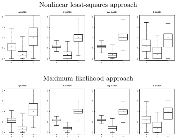
One fitting and model-selection pipeline, based on nonlinear least squares or maximum likelihood, applies to spatial ARCH, spatial GARCH, hybrid spatial GARCH, spatial log-GARCH, spatial E-GARCH, and ordinary time-series GARCH as edge cases.
The novel spatial GARCH and E-GARCH processes give spatial analogues of GARCH and EGARCH with additive and multiplicative variance dynamics, so volatility spillovers can be estimated and tested through the parameters $\rho$ and $\lambda$ in $W_1=\rho W_1^*$ and $W_2=\lambda W_2^*$.
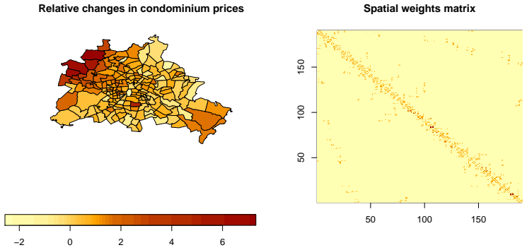
Because the observations $Y$ are uncorrelated with zero mean, the spatial GARCH-type processes can serve as error models inside spatial autoregressive regressions without contaminating the mean equation; this is exactly how the Berlin condominium example uses them.
In the paper's simulation study, likelihood-based model selection identifies the true model among the four variants in 92 to 99 percent of replications under the row-standardized and upper-triangular setting, and both estimators are roughly unbiased.
In the Berlin real estate application, an exponential spatial GARCH model fits the residuals of a spatial autoregressive model best, indicating local risk clusters that spill over to neighboring postal-code regions.

Reading between the lines

Editorial extensions of the paper, not claims the author makes directly.

Because the framework is a template over $(f,\gamma,g)$, the same estimator should carry threshold-GARCH and multivariate-GARCH variants; the paper names these as possible but does not develop them, so a direct extension is to instantiate the template and rerun the simulation study.
The Type I/Type II equivalence means model selection between spatial GARCH and spatial E-GARCH is effectively a choice between the identity link and the log link; one could estimate $f$ nonparametrically and let the data choose the dynamics, a route the paper flags only as future work.
The bounded-support assumption suggests that applying the model to heavy-tailed financial returns requires either truncating the innovation distribution or a different existence argument; a testable extension is to compare truncated-normal and $t$-distributed innovations on the same spatial grid and see when the fixed-point iteration breaks.

Share X Bluesky LinkedIn Reddit HN

Signed reviews

No signed human review yet.

Editorial analysis

A structured set of objections, weighed in public.

Desk editor's note, referee report, and a circularity audit.

Desk Editor's Note

read the letter

You should know this paper is the one to cite for a unified treatment of spatial GARCH-type models. It nests the spatial ARCH of Otto et al. and the Sato-Matsuda hybrid, and adds genuinely new spGARCH, E-spGARCH, and log-spGARCH processes. The syntax is clean: Y = diag(h)^{1/2}ε, with either F = α + W1γ(Y^(2)) + W2F (Type I) or F = α + W1g(ε) + W2F (Type II). All the examples drop out by choosing f and γ or g. The paper also gives a common estimation framework, an R package (spGARCH), simulations, and a Berlin real-estate application. That is a real contribution for practitioners.

The math mostly holds together. The existence proofs are contraction arguments and are fine as far as they go. The uncorrelatedness and symmetry results are standard. The NLSE and MLE sections are sketches rather than full proofs — the consistency argument is explicitly a sketch, and the claim that any KKT point is globally optimal for linear constraints is not true in general for nonconvex problems. Those are weaknesses, but not fatal; they can be fixed with more careful asymptotics.

The bigger soft spot is the spGARCH process itself. For Type I with f(x)=x, the solution is h = (I − W1E − W2)^{-1}α. That inverse can have negative entries if ρ(W1E+W2) ≥ 1, and with unbounded innovations this happens with positive probability for row-standardized symmetric weights. Theorem 1 only gives a sufficient contraction condition; the bounded-support assumption in Section 3.2.1 is mentioned but the bound needed for ρ ε² + λ < 1 is never stated or checked. The simulations dodge the issue by zeroing the upper triangle of W, making the process directional. The Berlin application uses a symmetric row-standardized contiguity matrix with t_3 innovations and estimates ρ=0.061, λ=0.209 — no existence check. So the flagship model may not be well-defined in the exact setting the application uses. That should be addressed head-on: either state the support bound, prove nonnegativity under weaker conditions, or restrict the model to directional weights where the issue disappears.

Who is this for? Anyone doing spatial econometrics or spatial statistics who wants a common language for volatility clustering. It is worth a serious referee; the framework is new and usable. But I'd want the spGARCH existence question cleared up before I trust the empirical results.

My recommendation: send it to peer review with a requirement that the authors either establish conditions for h ≥ 0 for symmetric weights or explicitly limit the model's domain, and tighten the NLSE/MLE asymptotics.

Referee Report

3 major / 5 minor

Summary. The paper proposes a unified spatial and spatiotemporal GARCH framework in which the observation vector satisfies Y = diag(h)^{1/2} ε, with h linked to F = f(h) through either a Type I specification (F = α + W1 γ(Y^{(2)}) + W2 F) or a Type II specification (F = α + W1 g(ε) + W2 F). Within this framework the authors place the existing spatial ARCH model of Otto et al. and the hybrid model of Sato and Matsuda, and they introduce new spatial GARCH, exponential GARCH, and logarithmic GARCH processes. They propose estimation by nonlinear least squares and maximum likelihood, study model selection via Monte Carlo simulations, and illustrate the methods on Berlin condominium price data after fitting a spatial autoregressive mean model. The paper also discusses the relationship between the Type I and Type II representations and provides partial derivatives of h needed for the likelihood Jacobian.

Significance. If the well-definedness issues are resolved, the unified framework is a valuable conceptual contribution: it nests several previously disparate spatial ARCH-type models and time-series GARCH models in one class, and it offers a common estimation and model-selection strategy. The explicit treatment of the Type I/Type II relationship, the availability of an R package, and the careful Monte Carlo comparison are concrete strengths. The empirical application to real estate prices demonstrates the practical motivation. However, the flagship spGARCH process is not shown to be well-defined for the symmetric row-standardized weight matrices used in the empirical application, and the asymptotic properties of the proposed estimators are only sketched, so the central claims need additional rigorous support.

major comments (3)

[Section 2.1.1, Theorem 1 and Example 2 (Eq. 4)] Theorem 1 asserts the existence of exactly one real-valued solution Y, but the proof only establishes a fixed point h of the contraction T in (3). It never verifies that all components of h are nonnegative, so the notation Y = diag(h)^{1/2}ε is not justified: if any h(s_i) < 0, Y is not real-valued. For the spGARCH model of Example 2, h solves h = (I - W1E - W2)^{-1}α, so h ≥ 0 requires (I - W1E - W2)^{-1}α ≥ 0. With W1, W2 nonnegative and α > 0, a sufficient condition is ρ(W1E + W2) < 1, but the paper neither states nor verifies this condition. The bounded-support assumption in Section 3.2.1 is not sufficient by itself: for row-standardized W* and W1 = ρW*, W2 = λW*, one needs ρ b^2 + λ < 1, where b is the bound on |ε|. The simulations in Section 4 explicitly use triangular weight matrices ('the upper diagonal elements were set to zero to avoid negative values of h(si)'), whereas the Berlin application in Section 5 uses a symmetric row-standardized contiguity matrix and t-distributed errors with 3 degrees of freedom; no check is reported for the fitted values ρ = 0.0609 and λ = 0.2093. Because the spGARCH process is the flagship new example of the unified framework, this gap is load-bearing.
[Section 3.2.1 (NLSE)] The consistency argument for the nonlinear least squares estimator is only a sketch and does not establish the claimed asymptotic properties as written. The decomposition of Q_n(ϑ) into In,...,VIIIn assumes E(log(ε(s_i)^2)) is a known constant c, yet c is not specified and depends on the unknown error distribution; in the application the error distribution is estimated (t with 3 d.f.), so c is unknown. The key step in the treatment of IVn, namely the expansion log(1 + κ d_i(λ)'Y^{(2)} / c_i(λ)) = κ (d_i(λ)'/c_i(λ))(Y^{(2)} - E Y^{(2)}) + o_p(1), requires a uniform integrability or boundedness condition that is not derived; the condition involving \tilde W Cov(Y^{(2)}) \tilde W' / n^2 → 0 is asserted without proof. If the NLSE is presented as a principal estimation method, the identification of ϑ0 and the uniform convergence of Q_n need to be proved under explicit regularity conditions.
[Section 3.2.2 (MLE)] The maximum likelihood section does not establish consistency or asymptotic normality of the ML estimator; it states that the Jacobian determinant has no explicit expression and that its properties are 'difficult to analyze.' The inverse function theorem is invoked without verifying the needed conditions on the support of ε (e.g., that the determinant of J is nonzero for almost every ε), and the transformation rule (14) is applied without discussing whether the map ε ↦ Y is a diffeomorphism on the relevant domain. Since the paper claims estimators are 'derived' for the common framework, the ML part should either provide a rigorous asymptotic treatment or explicitly state the consistency of the numerical MLE as an open conjecture supported only by simulations.

minor comments (5)

[Section 2.1.1, after Theorem 1] There is a typo: 'this result resents a possibility' should be 'this result represents a possibility.'
[Section 3.2.1, objective function] The displayed sum-of-squares formula has a missing closing parenthesis: it should be (H_i - log(h_ϑ(s_i)))^2, not (H_i - log(h_ϑ(s_i))2.
[Section 2.1.2, first paragraph] The phrase 'the the Type I and Type II approaches' contains a duplicated definite article.
[Table 2 and Section 5] The labels 'Ir res.' and 'Ir squ. res.' are unclear; they should be typeset as I_r for residuals and I_r for squared residuals, or given as full terms in the table caption.
[References] The reference to 'Newey, K. and McFadden, D.' should be corrected to 'Newey, W. K. and McFadden, D.'

Circularity Check

0 steps flagged · score 0.0 of 10

No significant circularity: the unified framework is introduced independently, and its examples are explicit special cases rather than fitted or predicted quantities.

full rationale

The paper's derivation chain is self-contained. The unified model is introduced directly through the general equations Y = diag(h)^{1/2} epsilon with Type I F = alpha + W1 gamma(Y^(2)) + W2 F and Type II F = alpha + W1 g(epsilon) + W2 F; Examples 1 through 5 then instantiate it by explicit choices of f, gamma, g, and the weight matrices, so the coverage claim is a definitional nesting rather than a relation fitted from the target quantities. The estimators in Section 3 are derived from the model equations using standard nonlinear least squares and likelihood arguments, and the Monte Carlo study in Section 4 simulates data from known models, so no fitted parameter is relabeled as a prediction. The Berlin application estimates parameters and selects models by BIC without presenting fitted values as out-of-sample predictions. Self-citations to Otto et al. (2016, 2018, 2019) and Otto (2019) are used for background, additional stochastic properties, and software implementation; existence and uniqueness are established by the paper's own Theorem 1 and Theorem 3 via Banach fixed-point and inverse-function arguments, not by the cited prior work. The limitation that simulations set the upper diagonal elements to zero to avoid negative values of h(si), together with the bounded-support assumption in Section 3.2.1, concerns whether h is real-valued; that is an existence and nonnegativity condition issue, not a circularity, because it does not make a derived result equal to its input by construction.

Assumptions & free parameters 7 free parameters · 6 assumptions · 0 invented entities

The paper's central framework relies on standard fixed-point and moment arguments, plus domain assumptions about spatial weight matrices and error symmetry. The restrictive assumptions are the bounded-support condition for spGARCH and the known constant in the NLSE, which are introduced to make the existence and estimation arguments work. No new physical or conceptual entities are postulated.

free parameters (7)

alpha = 0.1757 (spGARCH), 0.0000 (log-spGARCH), 2.8703 (E-spGARCH) in Berlin application
Intercept of the variance equation; estimated from data via NLSE or MLE. It is a model parameter, not an ad hoc constant, but it is fitted.
rho = 0.0609 / 0.0507 / 1.5339 in Berlin application
Coefficient for the W1 weight matrix, measuring shock spillover from neighboring locations; estimated from data.
lambda = 0.2093 / 0.9646 / 3.0380 in Berlin application
Coefficient for the W2 weight matrix, measuring volatility spillover from neighboring locations; estimated from data.
Theta = 0.5 in simulations, 1 in application
Asymmetry parameter of the E-spGARCH model; set by hand and treated as known rather than estimated.
zeta = 0
Leverage parameter of the E-spGARCH model; set to zero in both simulations and application.
b = 2
Exponent in the log-spGARCH model; set by hand and treated as known.
t-distribution degrees of freedom = 3 or 7 selected by BIC
Shape of the error distribution in the empirical application; selected by minimizing BIC.

assumptions (6)

domain assumption The error process epsilon is sign-symmetric, i.e., epsilon has the same distribution as ((-1)^{v1} epsilon(s1), ..., (-1)^{vn} epsilon(sn)) for all sign vectors.
Used in Theorems 2 and 4 to establish symmetry, zero odd moments, and uncorrelatedness of the observations. Standard for ARCH-type models.
domain assumption The weighting matrices W1 and W2 are non-negative with zero diagonal, and the matrix I-W2 (or I-W1-W2 for the hybrid model) is invertible.
Required for the existence of the process and for explicit solutions in Examples 2 through 5.
domain assumption The function f has an inverse on (0, infinity) and f^{-1} is convex for moment existence results.
Used in Theorem 4(a) to bound moments of Y via Jensen's inequality.
ad hoc to paper E(log(epsilon(si)^2)) is a known constant in the NLSE approach.
The estimation objective in Section 3.2.1 subtracts this constant, but the paper never estimates it; the user must supply it.
ad hoc to paper For the spGARCH model, the innovations epsilon have bounded support and the weight matrices are restricted, e.g., triangular, to ensure positive h and the contraction condition.
Section 3.2.1 and the simulation section impose this to guarantee existence and avoid negative variances; it is not derived from the model itself.
standard math The inverse function theorem applies to the transformation from epsilon to Y for the likelihood.
Used to obtain the likelihood in Section 3.2.2; the Jacobian is assumed non-singular.

how reviews work

0 comments

Cite this review

Pith. "Pith review of Spatial and Spatiotemporal GARCH Models -- A Unified Approach." pith.science (2026). https://pith.science/paper/M6LQY24T

@misc{pith2026190808320,
  author       = {Pith},
  title        = {Pith review of: Spatial and Spatiotemporal GARCH Models -- A Unified Approach},
  year         = {2026},
  howpublished = {\url{https://pith.science/paper/M6LQY24T}},
  note         = {Machine review of arXiv:1908.08320}
}

read the original abstract

In time-series analyses, particularly for finance, generalized autoregressive conditional heteroscedasticity (GARCH) models are widely applied statistical tools for modelling volatility clusters (i.e., periods of increased or decreased risk). In contrast, it has not been considered to be of critical importance until now to model spatial dependence in the conditional second moments. Only a few models have been proposed for modelling local clusters of increased risks. In this paper, we introduce novel spatial GARCH and exponential GARCH processes in a unified spatial and spatiotemporal GARCH-type model, which also covers all previously proposed spatial ARCH models as well as time-series GARCH models. For this common modelling framework, estimators are derived based on nonlinear least squares and on the maximum-likelihood approach. In addition to the theoretical contributions of this paper, we suggest a model selection strategy that is verified by a series of Monte Carlo simulation studies. Eventually, the use of the unified model is demonstrated by an empirical example that focuses on real estate prices from 1995 to 2014 across the ZIP-Code areas of Berlin. A spatial autoregressive model is applied to the data to illustrate how locally varying model uncertainties can be captured by the spatial GARCH-type models.

Figures

Figures reproduced from arXiv: 1908.08320 by the authors.

**Figure 3.** Relative changes (in per cent) of the Box-Cox transformed prices for all Berlin ZIP [PITH_FULL_IMAGE:figures/full_fig_p020_3.png] view at source ↗

**Figure 4.** Thus, spGARCH models can be used to analyze various forms of information, whether [PITH_FULL_IMAGE:figures/full_fig_p022_4.png] view at source ↗

Figures from the paper (1 more)

**Figure 4.** Figure 4: Financial network of selected stocks of the S&P 500, where the color of the nodes [PITH_FULL_IMAGE:figures/full_fig_p023_4.png]

Discussion (0). Continue with ORCID to comment.

Reference graph

Works this paper leans on

22 extracted references · 20 canonical work pages

[1]

Bollerslev, T. (1986). Generalized Autoregressive Conditional Heteroskedasticity . Journal of Econometrics , 31(3):307--327

work page 1986
[2]

Cressie, N. (1993). Statistics for Spatial Data . Wiley

1993
[3]

and Wikle, C

Cressie, N. and Wikle, C. K. (2011). Statistics for Spatio-Temporal Data . Wiley

work page 2011
[4]

Day, T. E. and Lewis, C. M. (1992). Stock market volatility and the information content of stock index options. Journal of Econometrics , 52(1-2):267--287

work page 1992
[5]

P., Lacombe, D

Elhorst, J. P., Lacombe, D. J., and Piras, G. (2012). On model specification and parameter space definitions in higher order spatial econometric models. Regional Science and Urban Economics , 42(1-2):211--220

work page 2012
[6]

Engle, R. F. (1982). Autoregressive Conditional Heteroscedasticity with Estimates of the Variance of United Kingdom Inflation . Econometrica: Journal of the Econometric Society , 50(4):987--1007

work page 1982
[7]

Engle, R. F. and Ng, V. K. (1993). Measuring and testing the impact of news on volatility. The Journal of Finance , 48(5):1749--1778

work page 1993
[8]

and Zakoian, J.-M

Francq, C. and Zakoian, J.-M. (2011). GARCH models: Structure, Statistical Inference and Financial Applications . John Wiley & Sons

work page 2011

Show all 22 references

[9]

Geweke, J. (1986). Comment on modelling the persistence of conditional variances. Econometric Reviews , (1):57--61

1986
[10]

Harville, D. A. (2008). Matrix Algebra from a Statistician's Perspective , volume 1. Springer

2008
[11]

Heynen, R., Kemna, A., and Vorst, T. (1994). Analysis of the term structure of implied volatilities. Journal of Financial and Quantitative Analysis , 29(1):31--56

1994
[12]

Lee, L.-F. (2004). Asymptotic Distributions of Quasi-Maximum Likelihood Estimators for Spatial Autoregressive Models . Econometrica , 72(6):1899--1925

2004
[13]

Milh j, A. (1987). A multiplicative parameterization of ARCH models . Universitetets statistiske Institut

1987
[14]

Nelson, D. B. (1991). Conditional heteroskedasticity in asset returns: A new approach. Econometrica: Journal of the Econometric Society , pages 347--370

1991
[15]

Otto, P. (2019). spGARCH : An R -package for spatial and spatiotemporal ARCH models. to appear in: The R Journal

2019
[16]

Otto, P., Schmid, W., and Garthoff, R. (2016). Generalized spatial and spatiotemporal autoregressive conditional heteroscedasticity. arXiv:1609.00711

2016 arXiv
[17]

Otto, P., Schmid, W., and Garthoff, R. (2018). Generalised Spatial and Spatiotemporal Autoregressive Conditional Heteroscedasticity . Spatial Statistics , 26:125--145

2018
[18]

Otto, P., Schmid, W., and Garthoff, R. (2019). Stochastic properties of spatial and spatiotemporal arch models. Statistical Papers

2019
[19]

Pantula, S. G. (1986). Comment on modelling the persistence of conditional variances. Econometric Reviews , 5(1):71--74

1986
[20]

and Matsuda, Y

Sato, T. and Matsuda, Y. (2017). Spatial autoregressive conditional heteroskedasticity models. Journal of the Japan Statistical Society , 47(2):221--236

2017
[21]

and Matsuda, Y

Sato, T. and Matsuda, Y. (2018a). Spatial GARCH models. Technical report, Graduate School of Economics and Management, Tohoku University

2018
[22]

and Matsuda, Y

Sato, T. and Matsuda, Y. (2018b). Spatiotemporal ARCH models. Technical report, Graduate School of Economics and Management, Tohoku University

2018

Pith tools

Reviewed August 14, 2026 · model on record in the stance chip above.

[1] [1]

Bollerslev, T. (1986). Generalized Autoregressive Conditional Heteroskedasticity . Journal of Econometrics , 31(3):307--327

work page 1986

[2] [2]

Cressie, N. (1993). Statistics for Spatial Data . Wiley

1993

[3] [3]

and Wikle, C

Cressie, N. and Wikle, C. K. (2011). Statistics for Spatio-Temporal Data . Wiley

work page 2011

[4] [4]

Day, T. E. and Lewis, C. M. (1992). Stock market volatility and the information content of stock index options. Journal of Econometrics , 52(1-2):267--287

work page 1992

[5] [5]

P., Lacombe, D

Elhorst, J. P., Lacombe, D. J., and Piras, G. (2012). On model specification and parameter space definitions in higher order spatial econometric models. Regional Science and Urban Economics , 42(1-2):211--220

work page 2012

[6] [6]

Engle, R. F. (1982). Autoregressive Conditional Heteroscedasticity with Estimates of the Variance of United Kingdom Inflation . Econometrica: Journal of the Econometric Society , 50(4):987--1007

work page 1982

[7] [7]

Engle, R. F. and Ng, V. K. (1993). Measuring and testing the impact of news on volatility. The Journal of Finance , 48(5):1749--1778

work page 1993

[8] [8]

and Zakoian, J.-M

Francq, C. and Zakoian, J.-M. (2011). GARCH models: Structure, Statistical Inference and Financial Applications . John Wiley & Sons

work page 2011