REVIEW 3 major objections 4 minor 36 references
Robust Navigation of a Soft Growing Robot by Exploiting Contact with the Environment
T0 review · 3 major / 4 minor · reviewed 2026-08-14 · deepseek-v4-flash
Pith's one-line read Soft growing robots navigate better by using obstacles as guides, not avoiding them.
desk verdict Credible incremental advance in soft-robot navigation, but the headline robustness claim is partly self-fulfilling and needs a physical check before it becomes a strong result. read the letter →
The pith
A machine-rendered reading of the paper's core claim, the machinery that carries it, and where it could break.
The reading
What carries the argument
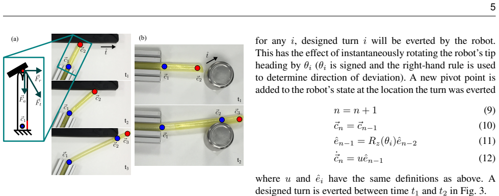
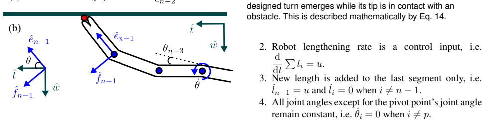
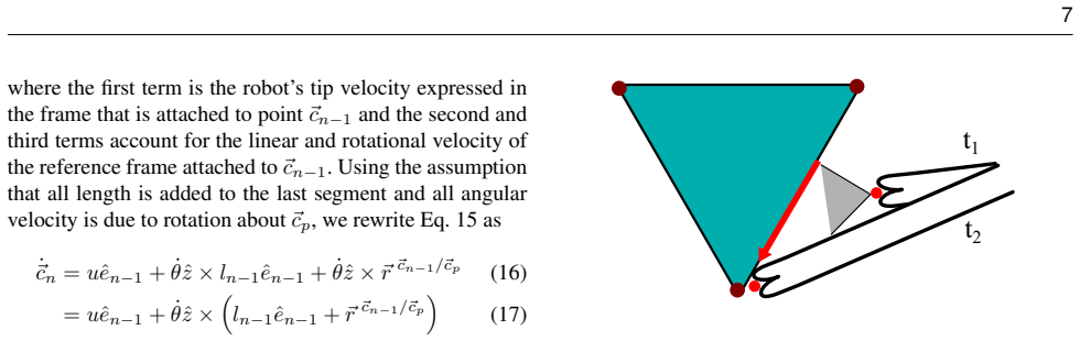
The key machinery is the obstacle interaction kinematic model: when the robot's tip contacts an obstacle, the tip is constrained to move parallel to the obstacle's tangent while the whole distal chain pivots about the most proximal unsupported pivot point that has the same handedness as the direction of turning. This differential kinematics (Eq. 18) determines how the robot's state changes during contact, and it is the mechanism that, in the planner, turns obstacles into passive guides that consolidate many possible paths into a single one. The planner also relies on a graph-based waypoint sequence generation where zero-weight edges correspond to obstacle-guided motion and weight-1 edges correspond to designed turns.
What would settle it
In a controlled physical experiment with chained obstacles (e.g., two or more walls in sequence), track the actual pivot point and tip trajectory with overhead cameras and compare to the model's prediction. If the tip systematically pivots about a point other than the most proximal unsupported same-handedness pivot, or if the tip fails to slide along the obstacle tangent under the stated pressure and material conditions (thin-walled polyethylene, low pressure, short free length), the model's core claim is refuted. Another direct falsifier: run the planner's numerical robustness test with a different, more detailed simulation (e.g., finite element or Cosserat rod) and see if the contact-exploiting design still outperforms the obstacle-avoiding design.
Extended reading notes
Core claim
The central discovery is that a planner that explicitly exploits obstacle contact produces paths that are more robust to uncertainty than a planner that avoids all obstacle contact. The paper formalizes a lumped-parameter kinematic model of a tip-everting soft robot interacting with planar obstacles, in which the robot's tip slides along an obstacle's tangent while pivoting about the most proximal unsupported pivot point of matching handedness. Using this model, the planner finds waypoint sequences that minimize the number of designed turns, and then optimizes turn angles and segment lengths to maximize the probability of reaching a goal under manufacturing noise. In numerical experiments with 10,000 Monte Carlo trials, the contact-exploiting design reaches the destination with significantly higher probability for all tested levels of angular uncertainty, and physical deployments confirm that the robot can reach goals even when map mismatch and manufacturing error are present.
Load-bearing premise
The whole planning method and the robustness comparison rest on the heuristic rule that when the robot's tip hits an obstacle, it pivots about the most proximal unsupported pivot point of the same handedness and slides along the obstacle's tangent, without deriving that from first-principles mechanics; if real robots pivot about a different point or slide differently, the planned paths and the simulated robustness advantage may not hold in practice.
Editorial extensions
If this is right
- If the model is right, a soft growing robot can be steered through cluttered environments with fewer manufactured turns, because obstacles do part of the steering.
- Robots designed with contact exploitation will be more reliable under manufacturing noise, since obstacle contact reduces path uncertainty.
- The same planning approach could be applied to any robot that passively conforms to obstacle contours, such as other continuum or snake-like robots.
- The hole-in-the-wall experiment shows a concrete strategy: when approach angle is uncertain, aim at the wall beside the hole rather than directly at the hole.
Reading between the lines
- The robustness advantage of contact exploitation likely grows with environmental cluttering, since more obstacles provide more passive guidance; a testable extension is measuring success probability versus obstacle density.
- The paper's single-obstacle contact model may transfer to soft grippers or manipulators that benefit from environmental constraints during manipulation, not just navigation.
- The planner's reliance on a greedy design optimization could be replaced by a global optimization of the whole turn sequence, which might yield even fewer turns or higher robustness in chained interactions.
- An observable we would expect if the model is correct: physical robots with thinner walls and lower pressure should match the predicted pivot behavior more closely, while thicker walls or higher pressure would show deviations, particularly in chained obstacle interactions.
Signed reviews
Editorial analysis
A structured set of objections, weighed in public.
Referee Report
Summary. This paper proposes an empirical kinematic model for a tip-everting soft growing robot interacting with planar obstacles, and a planner that exploits obstacle contact. The model represents the robot by pivot points; when the tip contacts an obstacle, the robot pivots about the most proximal unsupported pivot point with the same handedness as the turn direction and slides along the obstacle tangent. The planner first selects a minimum-turn waypoint sequence via a graph over obstacle vertices, then greedily constructs a robot design that maximizes the probability of reaching each waypoint under manufacturing uncertainty modeled as uniform noise on segment lengths and turn angles. The paper validates single-contact wall following and hole navigation, predicts exit locations in an obstacle course for seven starting orientations, and demonstrates physical deployments of planned designs in maze and forest environments. Monte Carlo simulations (Fig. 16(c)) show the contact-exploiting design has higher success probability than a nominal obstacle-avoiding design under manufacturing uncertainty, while Fig. 16(d) shows it is less robust to map uncertainty.
Significance. The idea of deliberately using obstacles as passive guides for soft growing robots is valuable and timely. If the robustness ordering holds physically, the approach reduces the number of manufactured turns and improves navigation reliability under manufacturing error, with direct relevance to search-and-rescue and inspection. The paper contributes a transparent, reproducible model-based planning pipeline, including particle-based optimization and Monte Carlo evaluation, and the physical experiments demonstrate that the planned contact-exploiting designs are deployable. However, the central quantitative claim—that contact exploitation is more robust than avoidance—is currently supported mainly by simulations that use the same interaction model inside both the planner and the evaluator, so the magnitude of the advantage, and even its sign, remains to be verified in physical comparative trials.
major comments (3)
- [Experimental Results, Fig. 16(c)] The robustness comparison is model-in-the-loop. Both the planner (Eq. 20, Algorithm 1) and the evaluation in Fig. 16(c) use the identical obstacle interaction model and the same uncertainty model (Eq. 7), so the numerical ordering is partly self-fulfilling: the contact-exploiting design is optimized under exactly the model used to score it. The physical deployments in Fig. 18 demonstrate feasibility, not comparative robustness. To support the abstract's claim, the authors should report a physical Monte Carlo comparison of both designs under manufacturing variability, or clearly argue why model error cancels in the comparison.
- [Planar Kinematic Model, 'Obstacle pivot point c_p'] The pivot-point selection rule is an asserted heuristic, not derived from mechanics. The paper's own conclusion states that when the buckling assumptions are violated, 'it could affect the tip predictions for multiple, chained obstacle interactions.' The planner's waypoint sequences and the Fig. 16(c) simulations rely on this rule precisely in chained interactions. If the real pivot point in a chained scenario is not the most proximal same-handed unsupported pivot, the planned designs and success probabilities can change. At minimum, the authors should perform a sensitivity analysis over plausible alternative pivot-selection rules, or provide physical data for chained multi-contact sequences.
- [Abstract and Fig. 16(d)] The abstract's claim of 'more robust to uncertainty' is unqualified, but Fig. 16(d) shows the obstacle-avoiding design is more robust to map uncertainty. The claim should be restricted to manufacturing/design uncertainty or combined with a map-uncertainty metric. Additionally, the free parameters sigma_theta, sigma_L, and d are hand-chosen; without empirical calibration, the absolute success levels in Fig. 16(c) should not be over-interpreted.
minor comments (4)
- [Robot Design Generation] The text says T is a discretization of [-pi_M, pi_M], but the allowable turn set was previously defined as [-theta_M, theta_M]; pi_M appears to be a typo.
- [Manufacturing Uncertainty, Eq. (7)] The notation U(l_i - sigma_L, l_i + sigma_L) and U(theta_i - sigma_theta, theta_i + sigma_theta) should state whether sigma_L and sigma_theta are absolute or relative to the nominal values, and how they are expected to be estimated in practice.
- [Algorithm 1] Line 5 discards samples not within d of waypoint x_{i-1}, and the same d is used as the goal radius in Eq. 19. It would help to clarify whether these two uses of d are intended to be identical and how d was chosen in the experiments.
- [Growth Through a Cluttered Environment] The obstacle course experiment validates exit-location prediction for seven starting orientations, but it does not test the planner's multi-turn designs; a sentence noting this distinction would prevent overgeneralization.
Circularity Check
The headline robustness advantage in Fig. 16(c) is evaluated with the same obstacle-interaction model and success metric used as the planner's optimization objective, making the quantitative claim partly self-fulfilling; physical deployments provide independent but qualitative support.
-
fitted input called prediction
[Planning Paths that Exploit Obstacles / Problem Definition (Eq. 19) and Experimental Results / Optimal Robot Design (Fig. 16(c))]
"The objective of this section is to produce a nominal robot design ... such that ... has a high expectation of reaching the destination: E(||⃗ xd−⃗ cn~||<d) ... where (⃗ c1~,...,⃗ cn~) is the deployed robot state computed using the obstacle interaction model. ... Fig. 16(c) compares the robustness of the two designs to uncertainty in their physical realizations. The data was generated by running 10000 Monte Carlo simulations ... A simulation was counted as a success if the robot tip ended within 5 cm of the destination and a failure otherwise."
The planner's design objective (Eq. 19) is exactly the probability that the deployed tip, computed with the obstacle interaction model, lies within distance d of the destination. The headline robustness comparison in Fig. 16(c) reports the same probability for the same model and the same manufacturing-noise distributions (Eq. 7). The design parameters are chosen by maximizing this sample-based success probability (Alg. 1), so Fig. 16(c) evaluates the optimized design on its own training objective rather than on an independent predictive test.
full rationale
The central non-circular content is the empirical obstacle-interaction model: wall-following, hole-in-wall, and cluttered-course experiments (Figs. 12-15) and physical maze/forest deployments (Fig. 18) are external to the planner's optimization and lend independent support. The circularity burden comes from Fig. 16(c): the optimizer searches turn angles and lengths using the model and uncertainty distributions, and the same model and distributions are then used to produce the reported success-probability advantage. That is a fitted-input-called-prediction pattern rather than a purely logical derivation. The model's pivot-point selection rule ('the most proximal unsupported pivot point that has the same handedness as the direction the robot will be turned') is an asserted ansatz, and the paper's own conclusion concedes that if buckling assumptions are violated 'it could affect the tip predictions for multiple, chained obstacle interactions,' which is exactly where the planner's advantage is demonstrated. Fig. 16(d) further shows the contact-exploiting design is less robust to map uncertainty, so the abstract's unqualified 'more robust to uncertainty' overstates the evidence. These factors make the central quantitative claim partly self-fulfilling, but the independent physical tests and the baseline comparison keep the paper from being fully circular; score 4.
Assumptions & free parameters
free parameters (4)
- sigma_theta =
2 degrees in numerical experiments
- sigma_l =
1.1 cm in numerical experiments
- d =
5 cm success radius in simulations
- Delta_theta =
uniform angular uncertainty range in Fig. 14(c)
assumptions (7)
- domain assumption The robot's body does not slide relative to the environment, and everted turn locations remain fixed during growth.
- domain assumption Obstacle Interaction Assumption 1: the tip velocity is parallel to the obstacle tangent while in contact.
- domain assumption Obstacle Interaction Assumptions 2-4: controlled growth rate, length added only to the last segment, and all other joint angles constant.
- ad hoc to paper The robot pivots about the most proximal unsupported pivot point with the same handedness as the turn direction.
- domain assumption Head-on contact leads to transverse buckling at the base under the stated pressure and membrane conditions, so the tip slides rather than bends.
- domain assumption Manufacturing errors are independent uniform random variables with half-widths sigma_L and sigma_theta.
- ad hoc to paper The nominal obstacle-avoiding design is a reasonable baseline for comparison.
Cite this review
Pith. "Pith review of Robust Navigation of a Soft Growing Robot by Exploiting Contact with the Environment." pith.science (2026). https://pith.science/paper/TKTMFWO6
@misc{pith2026190808645,
  author       = {Pith},
  title        = {Pith review of: Robust Navigation of a Soft Growing Robot by Exploiting Contact with the Environment},
  year         = {2026},
  howpublished = {\url{https://pith.science/paper/TKTMFWO6}},
  note         = {Machine review of arXiv:1908.08645}
}
read the original abstract
Navigation and motion control of a robot to a destination are tasks that have historically been performed with the assumption that contact with the environment is harmful. This makes sense for rigid-bodied robots where obstacle collisions are fundamentally dangerous. However, because many soft robots have bodies that are low-inertia and compliant, obstacle contact is inherently safe. As a result, constraining paths of the robot to not interact with the environment is not necessary and may be limiting. In this paper, we mathematically formalize interactions of a soft growing robot with a planar environment in an empirical kinematic model. Using this interaction model, we develop a method to plan paths for the robot to a destination. Rather than avoiding contact with the environment, the planner exploits obstacle contact when beneficial for navigation. We find that a planner that takes into account and capitalizes on environmental contact produces paths that are more robust to uncertainty than a planner that avoids all obstacle contact.
Figures


Figures from the paper (12 more)




Reference graph
Works this paper leans on
- [1]
-
[2]
IEEE Robotics and Automation Letters 2(3): 1413--1419
Coevoet E, Escande A and Duriez C (2017) Optimization-based inverse model of soft robots with contact handling. IEEE Robotics and Automation Letters 2(3): 1413--1419
work page 2017
-
[3]
The International Journal of Robotics Research 35(1-3): 161--185
Deimel R and Brock O (2016) A novel type of compliant and underactuated robotic hand for dexterous grasping. The International Journal of Robotics Research 35(1-3): 161--185
work page 2016
-
[4]
Technical Report D-3466, National Aeronautics and Space Adminstration (NASA)
Fichter W (1966) A theory for inflated thin-wall cylindrical beams. Technical Report D-3466, National Aeronautics and Space Adminstration (NASA)
work page 1966
-
[5]
In: IEEE International Conference on Robotics and Automation (ICRA)
Greer JD, Blumenschein LH, Okamura AM and Hawkes EW (2018) Obstacle-aided navigation of a soft growing robot. In: IEEE International Conference on Robotics and Automation (ICRA). pp. 4165--4172
work page 2018
-
[6]
In: IEEE International Conference on Robotics and Automation (ICRA)
Greer JD, Morimoto TK, Okamura AM and Hawkes EW (2017) Series pneumatic artificial muscles ( sPAMs ) and application to a soft continuum robot. In: IEEE International Conference on Robotics and Automation (ICRA). pp. 5503--5510
work page 2017
-
[7]
In: IEEE International Conference on Robotics and Automation (ICRA)
Hammond ZM, Usevitch NS, Hawkes EW and Follmer S (2017) Pneumatic reel actuator: Design, modeling, and implementation. In: IEEE International Conference on Robotics and Automation (ICRA). pp. 626--633
work page 2017
-
[8]
Science Robotics 2(8): eaan3028
Hawkes EW, Blumenschein LH, Greer JD and Okamura AM (2017) A soft robot that navigates its environment through growth. Science Robotics 2(8): eaan3028
work page 2017
Show all 36 references
-
[9]
Soft Robotics 2(4): 155--164
Katzschmann RK, Marchese AD and Rus D (2015) Autonomous object manipulation using a soft planar grasping manipulator. Soft Robotics 2(4): 155--164
2015
-
[10]
IEEE Transactions on Robotics and Automation 12(4): 566--580
Kavraki LE, Svestka P, Latombe JC and Overmars MH (1996) Probabilistic roadmaps for path planning in high-dimensional configuration spaces. IEEE Transactions on Robotics and Automation 12(4): 566--580
1996
-
[11]
Autonomous Robots 40(3): 537--560
Killpack MD, Kapusta A and Kemp CC (2016) Model predictive control for fast reaching in clutter. Autonomous Robots 40(3): 537--560
2016
-
[12]
Cambridge University Press
LaValle SM (2006) Planning algorithms. Cambridge University Press
2006
-
[13]
In: IEEE International Conference on Robotics and Automation
Liljeback P, Pettersen KY and Stavdahl O (2009) Modelling and control of obstacle-aided snake robot locomotion based on jam resolution. In: IEEE International Conference on Robotics and Automation. pp. 3807--3814
2009
-
[14]
IEEE/ASME Transactions on Mechatronics 17(6): 1158--1169
Liljeback P, Pettersen KY, Stavdahl and Gravdahl JT (2012) Snake robot locomotion in environments with obstacles. IEEE/ASME Transactions on Mechatronics 17(6): 1158--1169
2012
-
[15]
Communications of the ACM 22(10): 560--570
Lozano-P \'e rez T and Wesley MA (1979) An algorithm for planning collision-free paths among polyhedral obstacles. Communications of the ACM 22(10): 560--570
1979
-
[16]
AIAA Journal 1(7): 1652--1655
Masser P, Page R and Stoner W (1963) Deflections of an inflated circular-cylindrical cantilever beam. AIAA Journal 1(7): 1652--1655
1963
-
[17]
In: IEEE International Conference on Robotics and Automation (ICRA)
Melchior NA and Simmons R (2007) Particle RRT for path planning with uncertainty. In: IEEE International Conference on Robotics and Automation (ICRA). pp. 1617--1624
2007
-
[18]
In: IEEE/RSJ International Conference on Intelligent Robots and Systems (IROS)
Neppalli S, Jones B, McMahan W, Chitrakaran V, Walker I, Pritts M, Csencsits M, Rahn C and Grissom M (2007) Octarm-a soft robotic manipulator. In: IEEE/RSJ International Conference on Intelligent Robots and Systems (IROS). pp. 2569--2569
2007
-
[19]
In: Robotics Sciences and Systems Workshop: Revisiting Contact - Turning a problem into a solution
P \'a ll E, Sieverling A and Brock O (2017) Towards motion plans that react to contact events. In: Robotics Sciences and Systems Workshop: Revisiting Contact - Turning a problem into a solution
2017
-
[20]
In: IEEE International Conference on Robotics and Automation (ICRA)
Park W, Kim JS, Zhou Y, Cowan NJ, Okamura AM and Chirikjian GS (2005) Diffusion-Based Motion Planning for a Nonholonomic Flexible Needle Model . In: IEEE International Conference on Robotics and Automation (ICRA). pp. 4600--4605
2005
-
[21]
IEEE Transactions on Robotics 21(1): 1--17
Roh Sg and Choi HR (2005) Differential-drive in-pipe robot for moving inside urban gas pipelines. IEEE Transactions on Robotics 21(1): 1--17
2005
-
[22]
In: Experimental Robotics
Rucker DC and Webster RJ (2014) Mechanics of continuum robots with external loading and general tendon routing. In: Experimental Robotics. Springer, pp. 645--654
2014
-
[23]
Nature 521(7553): 467--475
Rus D and Tolley MT (2015) Design, fabrication and control of soft robots . Nature 521(7553): 467--475. doi:10.1038/nature14543
2015 doi
-
[24]
In: Robotics Sciences and Systems Workshop: Revisiting Contact - Turning a problem into a solution
Sieverling A, Eppner C and Brock O (2017) Exploiting contact for efficient motion planning under uncertainty. In: Robotics Sciences and Systems Workshop: Revisiting Contact - Turning a problem into a solution
2017
-
[25]
Transactions on Computational Intelligence and AI in Games 4(2): 144--148
Sturtevant N (2012) Benchmarks for grid-based pathfinding. Transactions on Computational Intelligence and AI in Games 4(2): 144--148
2012
-
[26]
IEEE control systems 12(1): 21--27
Suzumori K, Iikura S and Tanaka H (1992) Applying a flexible microactuator to robotic mechanisms. IEEE control systems 12(1): 21--27
1992
-
[27]
In: Advances in Neural Information Processing Systems
Thrun S (2000) Monte C arlo POMDP s. In: Advances in Neural Information Processing Systems. pp. 1064--1070
2000
-
[28]
IEEE Transactions on Robotics 24(1): 88--104
Transeth AA, Leine RI, Glocker C, Pettersen KY and Liljeb \"a ck P (2008) Snake robot obstacle-aided locomotion: Modeling, simulations, and experiments. IEEE Transactions on Robotics 24(1): 88--104
2008
-
[29]
Part I : general model of robot interacting with environment
Vukobratovi \'c MK and Potkonjak V (1999) Dynamics of contact tasks in robotics. Part I : general model of robot interacting with environment. Mechanism and Machine Theory 34(6): 923--942
1999
-
[30]
The International Journal of Robotics Research 29(13): 1661--1683
Webster RJ and Jones BA (2010) Design and Kinematic Modeling of Constant Curvature Continuum Robots: A Review . The International Journal of Robotics Research 29(13): 1661--1683
2010
-
[31]
IEEE Transactions on Robotics 30(4): 880--889
Yip MC and Camarillo DB (2014) Model-less feedback control of continuum manipulators in constrained environments. IEEE Transactions on Robotics 30(4): 880--889
2014
-
[32]
Journal of Field Robotics 2(3): 289--307
Zheng YF and Hemami H (1985) Mathematical modeling of a robot collision with its environment. Journal of Field Robotics 2(3): 289--307
1985
-
[33]
, " * write output.state after.block = add.period write newline
ENTRY address author booktitle chapter doi edition editor eid howpublished institution isbn journal key month note number organization pages publisher school series title type url volume year label extra.label sort.label short.list INTEGERS output.state before.all mid.sentence...
-
[34]
write newline
" write newline "" before.all 'output.state := FUNCTION n.dashify 't := "" t empty not t #1 #1 substring "-" = t #1 #2 substring "--" = not "--" * t #2 global.max substring 't := t #1 #1 substring "-" = "-" * t #2 global.max substring 't := while if t #1 #1 substring * t #2 gl...
-
[35]
, " * write output.state after.block = add.period write newline
ENTRY address archive author booktitle chapter doi edition editor eid eprint howpublished institution isbn journal key month note number organization pages publisher school series title type url volume year label INTEGERS output.state before.all mid.sentence after.sentence aft...
-
[36]
write newline
" write newline "" before.all 'output.state := FUNCTION n.dashify 't := "" t empty not t #1 #1 substring "-" = t #1 #2 substring "--" = not "--" * t #2 global.max substring 't := t #1 #1 substring "-" = "-" * t #2 global.max substring 't := while if t #1 #1 substring * t #2 gl...
Reviewed August 14, 2026 · model on record in the stance chip above.
Discussion (0). Continue with ORCID to comment.