REVIEW 3 major objections 6 minor 26 references
Strategic Insider Trading Equilibrium with a Non-fiduciary Market Maker
T0 review · 3 major / 6 minor · reviewed 2026-08-14 · deepseek-v4-flash
Pith's one-line read A non-fiduciary market maker who sets price by adding a fee proportional to cumulative order flow can earn expected profits comparable to or larger than a perfectly informed insider, while making prices more volatile than fundamentals…
desk verdict A genuine but conditional continuous-time extension of Kyle with a fee-charging market maker; the headline profit comparison is selected by the regulator's volatility cap rather than derived as an equilibrium outcome, yet the integral-equation derivation deserves refereeing. read the letter →
The pith
A machine-rendered reading of the paper's core claim, the machinery that carries it, and where it could break.
The reading
What carries the argument
The central object is the fee schedule $k_t=(T-t)\kappa$ embedded in the market maker's price rule $p_t=E[\tilde v \mid \mathcal{F}^y_t]+k_t y_t$. Because $k_t$ is positive and linear in cumulative order flow, the price is pushed above the fair value after buying pressure and below it after selling pressure; since the order flow $y_t$ mean-reverts around zero, the market maker systematically buys low and sells high. The insider's trading intensity $\beta_t$, defined by $dx_t=(\tilde v-p_t)\beta_t\,dt$, is the other half of the mechanism: the insider's optimal $\beta_t$ solves the integral equation in Theorem 1, and it declines as $\kappa$ grows. The paper's main analytical tool is the linear-filtering representation of the conditional expectation $m_t$, which gives the variance $V(t)=E[y_t^2]$ and the mean-square error $\gamma_t(\beta)$ in closed form; these feed directly into both profit functions.
What would settle it
Let a second market maker enter and undercut the fee by any positive amount; if the only subgame-perfect outcome is $\kappa=0$, then the profit-dominance result depends entirely on the assumed absence of fee competition and would not survive entry.
Extended reading notes
Core claim
The paper's central claim is that replacing the fiduciary price rule with a non-fiduciary one changes the economics of the single-insider auction model without destroying equilibrium. The market maker announces the price rule $p_t=E[\tilde v \mid \mathcal{F}^y_t]+k_t y_t$, with $k_t=(T-t)\kappa$; the insider still trades with intensity $\beta_t$ against his information advantage $\tilde v-p_t$. The expected profits are $J^M(\kappa,\beta)=w^M_0+\int_0^T(k_s^2 V(s)\beta_s+\kappa V(s))\,ds$ for the market maker and $J^I(\kappa,\beta)=w^I_0+\int_0^T\beta_s(\gamma_s(\beta)+k_s^2V(s))\,ds$ for the insider, so the fee adds a positive, order-flow-driven income for the market maker. The insider optimally trades more softly when $\kappa$ rises, but the market maker's fee income still dominates beyond a moderate threshold, which the paper's baseline calibration places around $\kappa=0.06$. The paper also derives the price variance $\operatorname{var}(p_t)=\operatorname{var}(m_t)+k_t^2 V(t)+2k_t\operatorname{cov}(m_t,y_t)$, which exceeds the fundamental-based variance, and constructs a regulator-observable relative-volatility measure $rv(t,\kappa)$ that ties $\kappa$ to a cap on price distortion.
Load-bearing premise
The whole result depends on the assumed price rule $p_t=E[\tilde v \mid \mathcal{F}^y_t]+(T-t)\kappa y_t$, with a single scalar $\kappa$ chosen by the market maker under a regulatory volatility cap; if market makers could undercut the fee, if the fee were nonlinear in order flow, or if the regulator's cap were tighter, the stated profit comparison and volatility result could fail.
Editorial extensions
If this is right
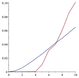
- A modest order-flow fee can make the market maker's expected profit exceed that of a perfectly informed insider; in the paper's baseline calibration the crossover occurs around $\kappa=0.06$.
- Speculative price volatility contains a fee-driven component $k_t^2 V(t)+2k_t\operatorname{cov}(m_t,y_t)$, so prices can be more volatile than fundamentals imply even without changes in dividend information.
- The insider trades less aggressively when the fee increases, but intensity rises again near the horizon as $k_t\to 0$, so the fee mainly shifts the timing and size of informed trading.
- A regulator can control the distortion by monitoring the relative volatility $rv(t,\kappa)$; a 15% cap in the baseline example keeps the market open for $\kappa$ up to about 0.07, and a 21% cap would allow $\kappa=0.09$.
- Price informativeness $\iota(t,\kappa)$ falls as $\kappa$ rises, so fee-driven price distortion makes prices less informative about fundamentals at every horizon.
Reading between the lines
- If the market maker's fee-setting power were subject to competition from a second market maker who could undercut $\kappa$ by a tiny amount, the profit-dominance result would likely shrink or vanish; the paper assumes a single market maker with regulatory protection, and testing that entry margin is a natural extension.
- The linear fee $k_t y_t$ is what makes the profit formulas tractable; a nonlinear fee such as a fee on absolute order flow would change the mean-reversion argument, and the ranking of market-maker versus insider profits might not survive.
- The model's volatility prediction is testable at the level of price impact: if the fee component is real, the coefficient of signed order flow on subsequent price changes should be positive and increasing in the market maker's market power, and the residual variance should exceed the variance implied by a fiduciary price.
- Because the fee is paid by both insider and noise traders, the model implies that noise traders bear the cost of intermediation; in an overlapping-generations or entry version, this could generate persistent wealth transfer to intermediaries, connecting to the paper's motivation.
Signed reviews
Editorial analysis
A structured set of objections, weighed in public.
Referee Report
Summary. This paper extends Kyle's (1985) continuous-time insider trading model by replacing the fiduciary market maker with a non-fiduciary market maker who sets prices according to pt = E[v|F_y] + (T−t)κ y_t. The insider's trading intensity β_t is characterized in Theorem 1 as a solution of an integral equation, and the paper derives closed-form expressions for the expected profits of the insider, the market maker, and the noise traders, as well as for the order-flow variance, relative volatility, and a price-informativeness measure. Numerical sections show that, as the fee parameter κ increases, the market maker's expected profit rises and eventually exceeds the insider's expected profit; the authors connect κ to a regulator-imposed cap on relative volatility rv*. The paper claims that setting a modest order-flow fee allows the market maker to earn profits of the same order as, or larger than, a perfectly informed insider, and that the model explains excess price volatility relative to fundamentals.
Significance. If the central claims were established, the paper would be a useful contribution to the literature on market power and intermediation in continuous-time insider trading: it provides explicit formulas for profits and price dynamics under a non-fiduciary price rule, and it frames a regulator's volatility cap as a constraint on the market maker's fee. The derivations in Section 3 and Appendix 1 are nontrivial, and the paper is transparent about several limitations, including the absence of an existence proof for the integral equation and the non-strategic treatment of the market maker. However, the headline profit comparison is currently presented as an unconditional result even though it is a consequence of an exogenously chosen regulatory threshold, and the technical optimality claim in Theorem 1 is not fully verified. With appropriate restatement and additional analysis, the continuous-time extension could be publishable.
major comments (3)
- [Section 4 and Appendix 1, Eq. (4.3)] Theorem 1 is derived as a first-order necessary condition, but the paper does not prove existence or uniqueness of a solution to the integral equation (4.3), nor does it show that the resulting β is a global maximizer of the insider's problem (4.2). The iterative procedure described in Section 7.2 is numerical, and no convergence argument is supplied, so the subsequent profit comparisons cannot be read as verified equilibrium outcomes. In addition, the displayed algebra is not internally consistent: the k^2 term appears with a plus sign in Eq. (10.3) and with a negative sign in Eq. (10.4), and the exponential factors in (10.4) do not obviously match the definition of V(t) used in the final expression (4.3). These points need to be fixed before the main theorem can be checked.
- [Appendix 2 and Section 3.3, Eq. (3.21)] Theorem 11.2 states that any Nash equilibrium has κ*=0 or κ*=K, never an interior 'modest' value. Combined with Eq. (3.21), which shows that JM is increasing in κ and grows without bound as κ→∞, an optimizing market maker would always choose the regulator's upper bound. The crossover near κ=0.06 reported in Section 7.4 is therefore not an equilibrium prediction of the model; it is an exogenous selection of the volatility cap. Table 2 confirms this cap-selection property: at rv*=1.08 the insider still earns pI=0.100 versus pM=0.060, while at rv*=1.15 the market maker earns pM=0.087 versus pI=0.055. The abstract and conclusion present the profit comparison unconditionally; this overstates what the model actually establishes.
- [Sections 6 and 9] The claim that the model 'indicates why speculative prices are more volatile than predicted by fundamentals' is not supported by the analysis as written. The model compares the market price p_t to the fair conditional price m_t; it does not compare prices to any fundamental process such as dividends or earnings. The numerical finding in Table 1 that var(p_t) exceeds var(m_t) is a statement about the distortion caused by the fee schedule relative to a fiduciary benchmark, not about excess volatility relative to fundamentals. The conclusion in Section 9 should be reformulated as a conditional statement about fee-induced price distortion.
minor comments (6)
- [Section 1] The reference to 'Campbell and Schiller (1988)' should be 'Campbell and Shiller (1988)'.
- [Section 3.2] The phrase 'by by the above observation' contains a duplicated 'by'.
- [Section 3.3, Eq. (3.23)] In the second exponential in Eq. (3.23), 'ke' appears where 'kr' is intended.
- [Section 7.1] The phrase 'Vi have' should be 'We have'.
- [Appendix 3] The reference to 'Theorem 3.2' appears to be an error; the intended reference is likely Theorem 11.2 in Appendix 2.
- [Section 5, Table 2] Table 2 reports profit values at t=9, while the text describes rv* as a supremum over t; the exact time convention used for the reported crossover should be stated explicitly.
Circularity Check
The headline profit comparison is cap-selection rather than equilibrium: JM grows in κ and Appendix 2 allows only corner κ, so the claim that the market maker can beat the insider is imposed by the regulator's 15% volatility cap, not derived as a prediction.
-
fitted input called prediction
[Abstract; Section 2 Eq. (2.2); Section 3.3 Eq. (3.21); Section 5 Table 2; Appendix 2 Theorem 11.2]
"by setting a modest fee conditional of the order flow, the market maker is able to obtain a profit of the order of magnitude, and even better than, a perfectly informed insider. ... (2.2) p_t =E[˜v +u_t|F^y_t ] :=m_t +E[u_t|F^y_t ], ... u_t =k_ty_t for k_t≥ 0 ... We assume that k_t = (T−t)κ ... (3.21) J_M(k,β ) =w^M_0 + ∫_0^T (k_s^2V(s)β_s +κV(s)) ds. ... rv∗ 1.15 κ∗ .070 pM(9,κ∗) .087 pI(9,κ∗) .055"
Equation (3.21) is monotonically increasing in κ, and the text states that the profit 'increases without bounds as ... κ→∞.' Hence the comparison 'market maker profit > insider profit' is not an equilibrium prediction but a choice of the free parameter κ. The paper's own Appendix 2, Theorem 11.2, says any Nash equilibrium has κ*=0 or κ*=K, never the interior 'modest' value 0.07 used for the headline. Table 2 makes the selection explicit: at rv*=1.08 the insider still wins (pI=0.100 vs pM=0.060), while at rv*=1.15 the market maker dominates (pM=0.087 vs pI=0.055). The claimed crossover near κ≈0.06 is therefore equivalent to assuming a 15% relative-volatility cap; if the regulator imposed a 10% cap the central conclusion would fail.
full rationale
The model's mathematical derivation is largely self-contained: the insider's integral equation (Theorem 1), the filtering equations, and the profit formulas are derived from stated assumptions, and the numerical examples are explicit about base-case parameters. The genuinely circular feature is in the presentation of the headline: because JM(k,β) grows without bound in κ and Appendix 2 shows equilibrium occurs only at a corner, the 'modest fee' comparison is selected by the exogenous regulator cap (rv*=1.15), not predicted by the theory. The self-citations to Aase-Gjesdal (2017/2018) and Aase et al. (2012) are used for standard filtering and order-form facts and are not load-bearing uniqueness claims. Thus the conditional contribution of the model remains valid, but the abstract's unconditional claim overstates what is established; the core profit comparison reduces by construction to the chosen cap.
Assumptions & free parameters
free parameters (5)
- κ (market maker fee intensity) =
0.025, 0.035, 0.045, 0.070, 0.090 in Table 2; κ around 0.06 to 0.07 for MM dominance in Section 7.4
- σ (noise trader volatility) =
0.20
- σ_v (prior standard deviation of asset value) =
0.30
- T (trading horizon) =
10
- rv* (regulator volatility threshold) =
1.15 (15% increase) in the main comparison; also 1.03, 1.05, 1.08, 1.21 in Table 2
assumptions (6)
- domain assumption The asset value v and the noise process B are Gaussian and independent; noise orders follow a Brownian motion with variance rate σ_t^2.
- domain assumption The insider restricts to order flow of the form dx_t=(v-p_t)β_t dt with deterministic β_t.
- domain assumption The market maker sets the price as p_t=E[v|F_y]+k_t y_t with k_t=(T-t)κ, κ≥0.
- domain assumption The terminal condition p_t converges to v as t approaches T holds, so the cross term in the insider's profit vanishes.
- domain assumption A regulator caps κ by imposing an upper bound on the relative volatility measure rv.
- standard math Kalman-Bucy filtering equations and the Riccati equation for the conditional error variance γ_t are applicable.
Cite this review
Pith. "Pith review of Strategic Insider Trading Equilibrium with a Non-fiduciary Market Maker." pith.science (2026). https://pith.science/paper/CDVSQLI5
@misc{pith2026190808777,
  author       = {Pith},
  title        = {Pith review of: Strategic Insider Trading Equilibrium with a Non-fiduciary Market Maker},
  year         = {2026},
  howpublished = {\url{https://pith.science/paper/CDVSQLI5}},
  note         = {Machine review of arXiv:1908.08777}
}
read the original abstract
The continuous-time version of Kyle's (1985) model is studied, in which market makers are not fiduciaries. They have some market power which they utilize to set the price to their advantage, resulting in positive expected profits. This has several implications for the equilibrium, the most important being that by setting a modest fee conditional of the order flow, the market maker is able to obtain a profit of the order of magnitude, and even better than, a perfectly informed insider. Our model also indicates why speculative prices are more volatile than predicted by fundamentals.
Figures


Figures from the paper (8 more)





Reference graph
Works this paper leans on
-
[1]
Aase, K. K. and F. Gjesdal (2017). ”Insider trading with non-fiduciary market makers.”. (Last version 2018) Discussion Paper FOR 8, Norwe- gian School of Economics
work page 2017
-
[2]
Aase, K. K. and B. Øksendal (2018). ”Strategic Insider Trading in Con- tinuous Time: A New Approach.” Discussion Paper FOR, Norwegian School of Economics. 9The result by Allinger and Mitter proved a long-standing conjecture by Kailath. 43
work page 2018
-
[3]
Aase, K., Bjuland, T. and Øksendal, B. (2012a). ”Partially informed liquidity traders.” Mathematics and Financial Economics 6, 93-104
work page 2012
-
[4]
Aase, K., Bjuland, T. and Øksendal, B. (2012b). ”Strategic Insider Trading Equilibrium: A Filter Theory Approach.” Afrika Matematika 23(2),145-162
work page 2012
-
[5]
Aase, K., Bjuland, T. and Øksendal, B. (2011). ”An anticipative linear filtering equation.” Systems & Control Letters 1-4
work page 2011
-
[6]
Admati, A. R. and Pfleiderer, P. (1988). ”A Theory of Intraday Patterns: Volume and Price Variability.”The Review of Financial Studies 1, 1, 3– 40
work page 1988
-
[7]
Allinger, D. F. and Mitter, S. K. (1981). ”New Results on the Innova- tions Problem for Non-Linear Filtering”. Stochastics 4, 339–348
work page 1981
-
[8]
Back, K. (1992). ”Insider Trading in Continuous Time”. The Review of Financial Studies Vol. 5, No 3, 387-409
work page 1992
Show all 26 references
-
[9]
Biagini, F., and Øksendal, B. (2005). ”A general stochastic calculus approach to insider trading”. Appl. Math. Optim. 52, 167–181
2005
-
[10]
Davis, M. H. A. (1977). Linear Estimation and Stochastic Control. Chapman and Hall
1977
-
[11]
Davis, M. H. A. (1984). Lectures on Stochastic Control and Nonlinear Filtering.. Tata Institute of Fundamental Research, Bombay
1984
-
[12]
Eide, I. B. (2007). ”An equilibrium model for gradually revealed asym- metric information”. Preprint, University of Oslo 6/2007
2007
-
[13]
R., and Milgrom, P
Glosten, L. R., and Milgrom, P. R. (1985). ”Bid, Ask and Transaction Prices in a Specialist Market with Hetrogeneously Informed Traders”. Journal of Financial Economics , 14, 71–100
1985
-
[14]
J., and Stiglitz, J
Grossman, S. J., and Stiglitz, J. E. (1980). ”On the Impossibility of Informationally Efficient Markets”. American Economic Review , 70 , 393–408. 44
1980
-
[15]
Holden, C. W. and Subrahmanyam, A. (1992). ”Long-Lived Private In- formation and Imperfect Competition”. The Journal of Finance, XLVII, 1 247–270
1992
-
[16]
Kallianpur, G. (1980). Stochastic Filtering Theory. Springer
1980
-
[17]
Kalman, R. E. (1960). ”A new approach to linear filtering and prediction problems”. J. Basic Engineering D 82, 35-45
1960
-
[18]
Schreve (1988)
Karatzas I., and S. Schreve (1988). Brownian motion and stochastic calculus. New York: Springer-Verlag
1988
-
[19]
Kyle, A. S. (1985). ”Continuous Auctions and Insider Trading”. Econo- metrica Vol.53, No. 6, 1315–1336
1985
-
[20]
Liptser, R. S. and Shiryaev, A. N.: Statistics of Random Processes II. Springer 1978
1978
-
[21]
Øksendal, B. (2013). ”Stochastic Differential Equations.” 6th Edition. Springer
2013
-
[22]
Russo, F., and Vallois, P. (1993). ”Forward, backward and symmetric stochastic integration”. Probab. Theory Related Fields 97, 403–421
1993
-
[23]
and Vallois, P
Russo, F. and Vallois, P. (1995). ”The generalized covariation process and Itˆ o formula”.Stoch. Process. Appl. 59, 81–104
1995
-
[24]
and Vallois, P
Russo, F. and Vallois, P. (2000). ”Stochastic calculus with respect to continuous finite quadratic variation processes”. Stoch. Stoch. Rep. 70, 1–40
2000
-
[25]
Tucker, H. G. (1967). A graduate course in probability. Academic Press, New York and London
1967
-
[26]
Yong, J. and X. Y. Zhou (1999). ”Hamiltonian Systems and the HJB Equations”. Springer-Verlag, New York, Inc. 45
1999
Reviewed August 14, 2026 · model on record in the stance chip above.
Discussion (0). Continue with ORCID to comment.