REVIEW 3 major objections 5 minor 45 references
Anomalous Kerr Effect in SrRuO$_3$ Thin Films
T0 review · 3 major / 5 minor · reviewed 2026-08-14 · deepseek-v4-flash
Pith's one-line read The Kerr-rotation bumps seen in SrRuO3 films come from magnetic-domain averaging over a non-monotonic Kerr-vs-magnetization curve, not from skyrmions.
desk verdict A fresh experimental observation that challenges skyrmion interpretations of Kerr/Hall bumps in SrRuO3, with a plausible domain-averaging mechanism whose quantitative case rests on one unmeasured input. read the letter →
The pith
A machine-rendered reading of the paper's core claim, the machinery that carries it, and where it could break.
The reading
What carries the argument
The load-bearing object is the local magnetization approximation (LMA): at optical frequencies the conductivity tensor is spatially local, so the measured Kerr angle is the spatial average of the Kerr angle of a uniform magnetization, θK(B) = x+(B)θK,U(M+(B)) + x−(B)θK,U(−M−(B)) in a two-domain picture. Its companion inputs are the experimentally extracted θK,U(M) curve, a polynomial fit to saturation Kerr data taken at different temperatures, and a tanh-based ansatz for the domain fraction x+(B) and domain magnetizations M±(B) fitted to the measured hysteresis loop. The LMA is checked against Kubo-formula supercell calculations for a cubic t2g model, agreeing for photon energies above roughly a quarter of the bandwidth; the d.c. Hall case is treated separately with an effective-medium approximation plus a domain-wall correction.
What would settle it
Measure the isothermal θK,U(M) at fixed temperature by an independent route, for example using a single-domain film or a spatially resolved Kerr microscope that images domains while sweeping field, and check whether the extracted curve is non-monotonic and whether the LMA average reproduces the bump's sign and height; if the isothermal curve is monotonic at 600 nm or the bumps persist in a single-domain sample, the proposed mechanism is ruled out.
Extended reading notes
Core claim
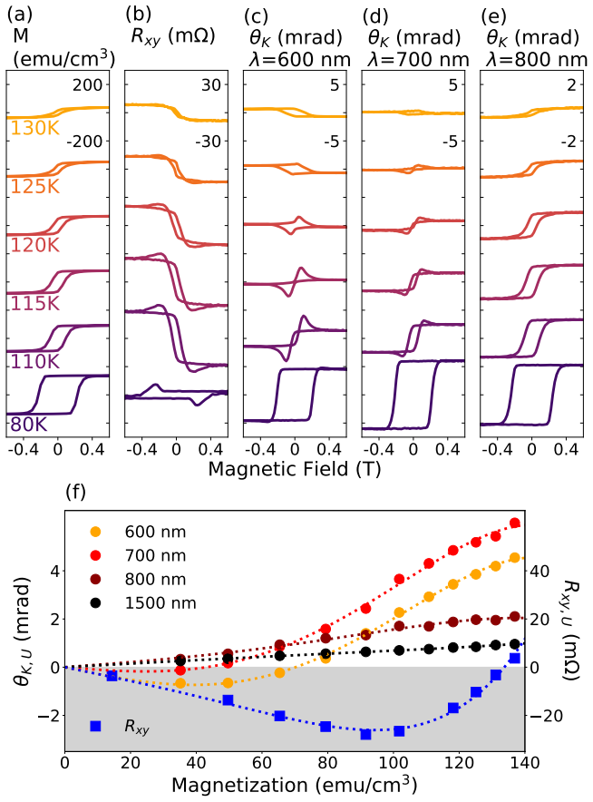
On the paper's own terms, the central discovery is an anomalous, bump-like contribution to the polar Kerr rotation in comparatively thick SrRuO3 films, where interfacial Dzyaloshinskii–Moriya interactions and skyrmions are not expected, and a controlled mechanism for it: measured Kerr rotation is the spatial average, over the sample, of the Kerr angle of a locally uniform magnetization, θK(B) = (1/V)∫θK,U(M(B,r))dr. Because θK,U(M) is non-monotonic, with a zero crossing and sign change as saturation magnetization is tuned by temperature, averaging over a two-domain distribution during reversal produces bumps whose sign, field position, temperature dependence, and resonant wavelength dependence match the data semi-quantitatively. The authors also show that a simple temperature-inhomogeneity model cannot produce positive Kerr bumps when the saturation signal decreases with temperature, and that an effective-medium average fails for the d.c. Hall signal; a domain-wall correction to the Hall conductivity, computed from a t2g model, has the right sign to account for the Hall anomalies.
Load-bearing premise
The calculation treats the saturation Kerr angle measured at different temperatures as the local isothermal Kerr angle inside one hysteresis loop, and the authors note in the supplemental material that quantitative agreement requires modifying this curve within plausible bounds; if that proxy is wrong, the predicted bump shape does not follow.
Editorial extensions
If this is right
- Bump-like MOKE features near coercivity do not by themselves indicate skyrmions or a topological Hall effect; they can be produced by nonlinear magneto-optics plus domain proliferation.
- The anomalous Kerr component should appear only at wavelengths and temperatures where θK,U(M) is strongly non-monotonic; at other wavelengths the Kerr signal should track M, as observed at 800 nm and 1500 nm.
- The same domain-averaging logic constrains interpretations of Hall anomalies: the effective-medium version fails for d.c. transport, so Hall bumps require either domain-wall contributions or a different microscopic mechanism.
- Strain and thickness control the anomaly: larger lattice mismatch gives larger and broader bumps, and only a finite thickness window shows them, tying the effect to the material's coercive and domain properties.
Reading between the lines
- A testable extension: a spatially resolving Kerr microscope that images domains during reversal should see the local Kerr angle follow the isothermal θK,U(M) curve, and the bump should vanish when the beam averages over a single domain.
- The same mechanism may apply to other ferromagnetic metals whose Kerr angle crosses zero as magnetization is tuned; such materials should show similar hysteresis-loop anomalies even with no topological texture.
- The domain-wall Hall calculation suggests a way to separate explanations: measurements of the Hall bump's dependence on domain-wall density, using patterned films or controlled field history, could distinguish domain-wall contributions from intrinsic topological Hall effect.
Signed reviews
Editorial analysis
A structured set of objections, weighed in public.
Referee Report
Summary. The paper reports magneto-optical Kerr effect (MOKE) measurements on SrRuO3 thin films (30–200 nm, with a focus on an 88 nm film on LSAT) and identifies bump-like anomalies in the Kerr rotation near the coercive field at certain wavelengths and temperatures, while the magnetization exhibits conventional hysteresis loops. The authors propose that these anomalies arise from a combination of a non-monotonic dependence of the Kerr angle on uniform magnetization, θK,U(M), and spatial averaging over magnetic domains during magnetization reversal. They introduce a local magnetization approximation (LMA), fit the measured magnetization to a two-domain model, and compute the Kerr loop as a weighted average of θK,U evaluated at the domain magnetizations. The predicted loops show qualitative agreement with the measured loops at 115 K and 120 K for λ = 600 nm. The paper also includes a numerical benchmark of the LMA against exact Kubo formula results for a t2g model with inhomogeneous magnetization, and a separate discussion of domain-wall corrections to the dc Hall conductivity.
Significance. If the proposed mechanism is correct, the paper challenges the commonly invoked skyrmion interpretation of anomalous Hall and MOKE features in SrRuO3 and offers a general, domain-based explanation for MOKE anomalies in ferromagnetic thin films. The numerical validation of the LMA against exact Kubo results in SM S5 is a valuable methodological contribution that strengthens the plausibility of the high-frequency averaging scheme. The paper is also notable for explicitly addressing alternative models of the Hall anomalies (SM S4) and for providing a specific, falsifiable prediction: the anomalies should appear only when θK,U(M) is non-monotonic and when magnetic domains proliferate. However, the central quantitative input, the isothermal θK,U(M) curve, is not directly measured, and the authors acknowledge in SM S7 that quantitative agreement requires modifying this curve within plausible but unquantified bounds. The significance is therefore conditional on an independent determination or first-principles support for the isothermal non-monotonic behavior.
major comments (3)
- [SM S7; main text, Fig. 4(d)] The model requires an isothermal θK,U(M) curve, but the input is extracted from saturation Kerr data taken at different temperatures, which bundles the temperature dependence of the optical response with the magnetization dependence. Because the sign, size, and even presence of the predicted bump are controlled by the non-monotonic part of θK,U(M), the central claim is not fully supported unless an isothermal non-monotonic relation is independently established. The modified curves in Fig. 12 of SM S7 are only constrained to terminate at the experimental data points for each temperature, which is a weak constraint, so the improved agreement in panels (d) and (g) does not, by itself, confirm the mechanism. The authors should either provide a direct isothermal measurement, a first-principles calculation of θK,U(M), or a quantitative sensitivity analysis showing that plausible isothermal curves within experimental uncertainties reproduce the observed bumps.
- [SM S6; main text, Fig. 4(a)–(c)] The two-domain magnetization fit introduces a flexible tanh ansatz with parameters b, w, b′, w′, δ, and ζ, and the computed Kerr loops depend directly on the fitted M±(B) through θK,U. The claim that the results are robust against variations in the precise shape of M−(B>0) is not demonstrated quantitatively. A sensitivity analysis with error bars on the extracted M±(B), or a comparison using a different functional form for M−(B), is needed to show that the predicted bumps are not an artifact of the flexible domain ansatz. This is important because the same fitted functions are used both for the magnetization and for the Kerr calculation.
- [Main text, Fig. 5 and conclusion] The LMA theory is compared with experiment for only two temperatures (115 K and 120 K) and one wavelength (600 nm), yet the abstract and conclusion claim a mechanism for anomalies observed over wide ranges of wavelength, temperature, and film thickness. The paper should either extend the LMA comparison to additional temperatures and wavelengths (for example, the 700 nm data where anomalies are also present), or explicitly temper the scope of the claim so that the quantitative theory is presented as demonstrated only at the two temperatures shown, while the broader data are interpreted through the more phenomenological θK,A decomposition.
minor comments (5)
- [SM S6, Eq. (10)] The parameter δ in the envelope function (B/B∗)δ is introduced but not defined in the main text; please define it at first use and give its fitted value for the reported temperatures.
- [Main text, Fig. 1(f) caption] The notation θK,U(T) is used before the subscript U is defined in the text; define 'U' (uniform) in the caption or earlier in the text.
- [Main text, Fig. 2] The color scale in Fig. 2(b) is labeled in units of θK,A, but the caption does not state the units explicitly; add '(mrad)' to the color bar label.
- [SM S3] The oblique-incidence data show that the p- and s-polarized signals are not related by a single overall factor, which the authors tentatively attribute to in-plane magnetization. This point is not discussed further; a sentence on its implications for the LMA or for the magnetization geometry would help.
- [Main text, abstract and conclusion] The phrase 'wide regimes of wavelength, temperature, and magnetic field' could be misread as implying the anomalies appear at all measured wavelengths; the data show they appear only for certain wavelengths (e.g., 600 nm and 700 nm, not 800 nm or 1500 nm). Consider rephrasing to 'wide regimes of temperature and magnetic field, with a strong wavelength dependence.'
Circularity Check
No significant circularity: the Kerr-anomaly explanation is a forward model built from measured magnetization hysteresis and measured high-field saturation Kerr data, not a fit to the target anomaly.
full rationale
The derivation chain is a forward model rather than a circular reduction. The two-domain parameters x+(B), M+(B), and M-(B) are fitted to the independently measured magnetization hysteresis loop (Fig. 4(a)-(c); SM S6), not to the Kerr signal. The function θK,U(M) is measured in the saturated, uniformly magnetized state at high field while temperature tunes M (Fig. 1(f); Fig. 4(d)); this curve does not contain the loop-anomaly information by construction. The predicted Kerr loop is then computed as θK(B) = x+(B)θK,U(M+(B)) + x-(B)θK,U(-M-(B)), i.e., by averaging a measured local response over field-dependent domain fractions. The qualitative bump appears already with the unmodified measured θK,U(M), as shown in Fig. 5, so the central claim does not reduce to a fit of the anomaly. SM S5 independently tests the local magnetization approximation against exact Kubo-formula conductivity for inhomogeneous Weiss-field profiles, finding agreement for large frequencies; no load-bearing self-citation is involved. The limitation admitted in SM S7 — that the model ultimately requires an isothermal θK,U(M) curve, which is beyond the scope of the study — is an acknowledged missing-input and sensitivity caveat, not circularity: the modified curves are presented as plausible deviations, are pinned at the measured saturation points, and the qualitative mechanism does not depend on them. The minor self-citation Ref. [32] for Tc~150 K is peripheral and not load-bearing. No step defines its output in terms of its input or renames a fitted parameter as a prediction.
Assumptions & free parameters
free parameters (3)
- Domain fraction ansatz parameters (b, w, δ) =
not stated in text
- Minority domain magnetization ansatz parameters (b', w', ζ) =
not stated in text
- Polynomial fit to θK,U(M) =
coefficients not stated
assumptions (4)
- standard math Kubo formula for the optical conductivity tensor
- domain assumption Local magnetization approximation (LMA): the Kerr angle of an inhomogeneous film equals the spatial average of the uniform Kerr angle θK,U(M(r))
- ad hoc to paper The two-domain model with tanh ansatz captures the domain evolution during magnetization reversal
- ad hoc to paper The saturation Kerr angle vs magnetization measured across temperatures is a valid proxy for the isothermal θK,U(M) needed inside a hysteresis loop
Cite this review
Pith. "Pith review of Anomalous Kerr Effect in SrRuO$_3$ Thin Films." pith.science (2026). https://pith.science/paper/KFBAJXHM
@misc{pith2026190808974,
  author       = {Pith},
  title        = {Pith review of: Anomalous Kerr Effect in SrRuO$_3$ Thin Films},
  year         = {2026},
  howpublished = {\url{https://pith.science/paper/KFBAJXHM}},
  note         = {Machine review of arXiv:1908.08974}
}
abstract
We study the magneto-optical Kerr effect (MOKE) in SrRuO$_3$ thin films, uncovering wide regimes of wavelength, temperature, and magnetic field where the Kerr rotation is not simply proportional to the magnetization but instead displays two-component behavior. One component of the MOKE signal tracks the average magnetization, while the second "anomalous" component bears a resemblance to anomalies in the Hall resistivity which have been previously reported in skyrmion materials. We present a theory showing that the MOKE anomalies arise from the non-monotonic relation between the Kerr angle and the magnetization, when we average over magnetic domains which proliferate near the coercive field. Our results suggest that inhomogeneous domain formation, rather than skyrmions, may provide a common origin for the observed MOKE and Hall resistivity anomalies.
Figures


Figures from the paper (13 more)


Reference graph
Works this paper leans on
-
[1]
D. J. Thouless, M. Kohmoto, M. P. Nightingale, and M. den Nijs, Phys. Rev. Lett. 49, 405 (1982)
1982
-
[2]
A. P. Schnyder, S. Ryu, A. Furusaki, and A. W. W. Ludwig, Phys. Rev. B 78, 195125 (2008)
2008
-
[3]
Kitaev, AIP Conference Proceedings 1134, 22 (2009)
A. Kitaev, AIP Conference Proceedings 1134, 22 (2009)
2009
-
[4]
S. Ryu, A. P. Schnyder, A. Furusaki, and A. W. W. Ludwig, New Journal of Physics 12, 065010 (2010)
2010
-
[5]
Nagaosa, J
N. Nagaosa, J. Sinova, S. Onoda, A. H. MacDonald, and N. P. Ong, Rev. Mod. Phys. 82, 1539 (2010)
2010
-
[6]
Z. Fang, N. Nagaosa, K. S. Takahashi, A. Asamitsu, R. Mathieu, T. Ogasawara, H. Yamada, M. Kawasaki, Y. Tokura, and K. Terakura, Science 302, 92 (2003)
2003
-
[7]
X. Wan, A. M. Turner, A. Vishwanath, and S. Y. Savrasov, Phys. Rev. B 83, 205101 (2011)
2011
-
[8]
H. Yang, Y. Sun, Y. Zhang, W.-J. Shi, S. S. P. Parkin, and B. Yan, New Journal of Physics 19, 015008 (2017)
2017
Show all 45 references
-
[9]
K¨ ubler and C
J. K¨ ubler and C. Felser, EPL (Europhysics Letters)108, 67001 (2014)
2014
-
[10]
Y. Chen, D. L. Bergman, and A. A. Burkov, Phys. Rev. B 88, 125110 (2013)
2013
-
[11]
Neubauer, C
A. Neubauer, C. Pfleiderer, B. Binz, A. Rosch, R. Ritz, P. G. Niklowitz, and P. B¨ oni, Phys. Rev. Lett. 102, 186602 (2009)
2009
-
[12]
M. Lee, W. Kang, Y. Onose, Y. Tokura, and N. P. Ong, Phys. Rev. Lett. 102, 186601 (2009). 32
2009
-
[13]
Kanazawa, Y
N. Kanazawa, Y. Onose, T. Arima, D. Okuyama, K. Ohoyama, S. Wakimoto, K. Kakurai, S. Ishiwata, and Y. Tokura, Phys. Rev. Lett. 106, 156603 (2011)
2011
-
[14]
Soumyanarayanan, M
A. Soumyanarayanan, M. Raju, A. L. Gonzalez Oyarce, A. K. C. Tan, M.-Y. Im, A. P. Petrovi´ c, P. Ho, K. H. Khoo, M. Tran, C. K. Gan, F. Ernult, and C. Panagopoulos, Nat. Mater. 16, 898 (2017)
2017
-
[15]
Legrand, J.-Y
W. Legrand, J.-Y. Chauleau, D. Maccariello, N. Reyren, S. Collin, K. Bouzehouane, N. Jaouen, V. Cros, and A. Fert, Sci. Adv. 4, eaat0415 (2018)
2018
-
[16]
J. A. Garlow, S. D. Pollard, M. Beleggia, T. Dutta, H. Yang, and Y. Zhu, Phys. Rev. Lett. 122, 237201 (2019)
2019
-
[17]
Kurumaji, T
T. Kurumaji, T. Nakajima, M. Hirschberger, A. Kikkawa, Y. Yamasaki, H. Sagayama, H. Nakao, Y. Taguchi, T.-h. Arima, and Y. Tokura, Science 365, 914 (2019)
2019
-
[18]
Matsuno, N
J. Matsuno, N. Ogawa, K. Yasuda, F. Kagawa, W. Koshibae, N. Nagaosa, Y. Tokura, and M. Kawasaki, Sci. Adv. 2, e1600304 (2016)
2016
-
[19]
K.-Y. Meng, A. S. Ahmed, M. Ba´ cani, A.-O. Mandru, X. Zhao, N. Bagu´ es, B. D. Esser, J. Flores, D. W. McComb, H. J. Hug, and F. Yang, Nano Lett. 19, 3169 (2019)
2019
-
[20]
B. Pang, L. Zhang, Y. B. Chen, J. Zhou, S. Yao, S. Zhang, and Y. Chen, ACS Applied Materials & Interfaces 9, 3201 (2017)
2017
-
[21]
Ohuchi, J
Y. Ohuchi, J. Matsuno, N. Ogawa, Y. Kozuka, M. Uchida, Y. Tokura, and M. Kawasaki, Nat. Commun. 9, 1 (2018)
2018
-
[22]
L. Wang, Q. Feng, Y. Kim, R. Kim, K. H. Lee, S. D. Pollard, Y. J. Shin, H. Zhou, W. Peng, D. Lee, W. Meng, H. Yang, J. H. Han, M. Kim, Q. Lu, and T. W. Noh, Nature Materials 17, 1087 (2018)
2018
-
[23]
Q. Qin, L. Liu, W. Lin, X. Shu, Q. Xie, Z. Lim, C. Li, S. He, G. M. Chow, and J. Chen, Advanced Materials 31, 1807008 (2019)
2019
-
[24]
D. Kan, T. Moriyama, K. Kobayashi, and Y. Shimakawa, Phys. Rev. B 98, 180408 (2018)
2018
-
[25]
Gerber, Phys
A. Gerber, Phys. Rev. B 98, 214440 (2018)
2018
-
[26]
L. Wang, Q. Feng, H. G. Lee, E. K. Ko, Q. Lu, and T. W. Noh, Nano Lett. 20, 2468 (2020)
2020
-
[27]
Malsch, D
G. Malsch, D. Ivaneyko, P. Milde, L. Wysocki, L. Yang, P. H. M. van Loosdrecht, I. Lindfors- Vrejoiu, and L. M. Eng, ACS Applied Nano Materials 3, 1182 (2020)
2020
-
[28]
Z. Q. Qiu and S. D. Bader, Review of Scientific Instruments 71, 1243 (2000)
2000
-
[29]
Huang, G
B. Huang, G. Clark, E. Navarro-Moratalla, D. R. Klein, R. Cheng, K. L. Seyler, D. Zhong, 33 E. Schmidgall, M. A. McGuire, D. H. Cobden, W. Yao, D. Xiao, P. Jarillo-Herrero, and X. Xu, Nature 546, 270 (2017)
2017
-
[30]
C. Gong, L. Li, Z. Li, H. Ji, A. Stern, Y. Xia, T. Cao, W. Bao, C. Wang, Y. Wang, Z. Q. Qiu, R. J. Cava, S. G. Louie, J. Xia, and X. Zhang, Nature 546, 265 (2017)
2017
-
[31]
P. N. Argyres, Phys. Rev. 97, 334 (1955)
1955
-
[32]
Z. Li, S. Shen, Z. Tian, K. Hwangbo, M. Wang, Y. Wang, F. M. Bartram, L. He, Y. Lyu, Y. Dong, G. Wan, H. Li, N. Lu, J. Zang, H. Zhou, E. Arenholz, Q. He, L. Yang, W. Luo, and P. Yu, Nat. Commun. 11, 184 (2020)
2020
-
[33]
normal contribution
for data on other films. We have measured the Kerr rotation in these films using a wavelength-tunable pulsed laser (repetition rate: 80 MHz) reduced to low-power ( <1 mW) and focused weakly onto a∼50µm spot on the sample, with the reflected beam modulated by a photo-elastic modul...
-
[34]
non-intrinsic
See Supplemental Material for details of: (i) additional MOKE data for the 88nm sample at different laser frequencies, (ii) further MOKE data on different thickness films on STO and LSAT substrates, (iii) MOKE measurements at oblique incidence, (iv) discussion of why an alternati...
-
[35]
M. Raju, A. Yagil, A. Soumyanarayanan, A. K. C. Tan, A. Almoalem, F. Ma, O. M. Auslaen- der, and C. Panagopoulos, Nat. Commun. 10, 696 (2019)
2019
-
[36]
Zahradn´ ık, K
M. Zahradn´ ık, K. Uhl´ ıˇ rov´ a, T. Maroutian, G. Kurij, G. Agnus, M. Veis, and P. Lecoeur, Materials and Design 187, 108390 (2020)
2020
-
[37]
D. J. Singh, Journal of Applied Physics 79, 4818 (1996)
1996
-
[38]
Liu and L
J. Liu and L. Balents, Phys. Rev. Lett. 119, 087202 (2017)
2017
-
[39]
X. Li, C. Collignon, L. Xu, H. Zuo, A. Cavanna, U. Gennser, D. Mailly, B. Fauqu´ e, L. Balents, Z. Zhu, and K. Behnia, Nat. Commun. 10, 3021 (2019)
2019
-
[40]
Koster, L
G. Koster, L. Klein, W. Siemons, G. Rijnders, J. S. Dodge, C.-B. Eom, D. H. A. Blank, and M. R. Beasley, Rev. Mod. Phys. 84, 253 (2012)
2012
-
[41]
Mahan, Many-Particle Physics, Physics of Solids and Liquids (Springer US, 2000); P
G. Mahan, Many-Particle Physics, Physics of Solids and Liquids (Springer US, 2000); P. Cole- man, Introduction to many-body physics (Cambridge University Press, 2015); D. J. Scalapino, S. R. White, and S. Zhang, Phys. Rev. B 47, 7995 (1993)
1993
-
[42]
Kostic, Y
P. Kostic, Y. Okada, N. C. Collins, Z. Schlesinger, J. W. Reiner, L. Klein, A. Kapitulnik, 34 T. H. Geballe, and M. R. Beasley, Phys. Rev. Lett. 81, 2498 (1998)
1998
-
[43]
J. S. Dodge, C. P. Weber, J. Corson, J. Orenstein, Z. Schlesinger, J. W. Reiner, and M. R. Beasley, Phys. Rev. Lett. 85, 4932 (2000)
2000
-
[44]
Stroud, Phys
D. Stroud, Phys. Rev. B 12, 3368 (1975)
1975
-
[45]
Granovsky, A
A. Granovsky, A. Vedyayev, and F. Brouers, Journal of Magnetism and Magnetic Materials 136, 229 (1994). 35
1994
Reviewed August 14, 2026 · model on record in the stance chip above.
Discussion (0). Continue with ORCID to comment.