Creation of digital elevation models for river floodplains

Alexander Khoperskov; Anna Klikunova

REVIEW 3 major objections 5 minor 23 references

Creation of digital elevation models for river floodplains

T0 review · 3 major / 5 minor · reviewed 2026-08-14 · deepseek-v4-flash

Challenge this review Re-run · record.json Download PDF Read on arXiv ↗ Review JSON

Pith's one-line read The paper argues that observed shorelines of ephemeral floodplain lakes are elevation contours, and feeding them into an iterative SRTM-based correction loop with hydrodynamic verification significantly improves the floodplain digital…

desk verdict Plausible DEM-refinement workflow whose improvement claim is unvalidated; the waterline-as-contour assumption needs an error analysis and independent ground truth. read the letter →

arxiv 1908.09005 v1 pith:DYEEHPPT submitted 2019-08-18 cs.CV eess.IVphysics.geo-ph

Anna Klikunova , Alexander Khoperskov This is my paper · ORCID

classification cs.CVeess.IVphysics.geo-ph

keywords digitalelevationmodelfloodplainmappingVolga-AkhtubainterfluvecoastlinedynamicsshallowwaterequationsSRTMmorphostructuralanalysisiterativedataassimilation

verification ladder T0 review T1 audit T2 compute T3 formal

The pith

A machine-rendered reading of the paper's core claim, the machinery that carries it, and where it could break.

The reading

This paper tries to establish a practical way to build a much more accurate digital elevation model of a flat river floodplain than the SRTM satellite grid alone provides, using the flat valley between the Volga and Akhtuba rivers as the test case. The key idea is that every observed coastline of a temporary flood lake is, to high accuracy, a contour line of the terrain, so a time series of coastlines from the spring flood supplies many local elevation constraints. These constraints are merged with river-depth soundings, channel vectorization, and morphostructural artifact checks through an iterative correction scheme, and the resulting model is checked by shallow-water hydrodynamic simulations of the flood. If the procedure works, floodplain topography can be updated and refined at low cost whenever flood imagery is available, which matters because flood forecasting and hydrological decision support depend on DEM quality.

What carries the argument

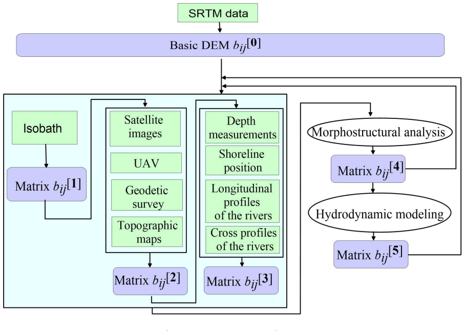
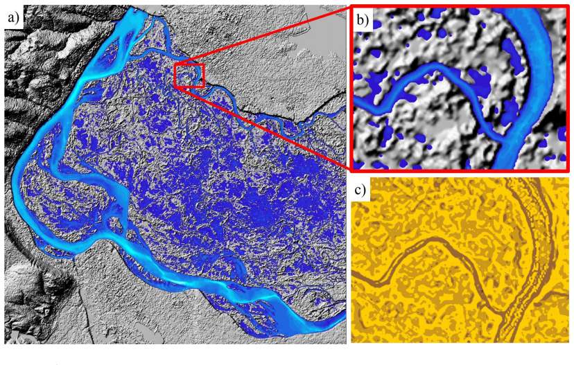
The load-bearing mechanism is the coastline-isoline identity: the waterline of a transient flood reservoir is treated as an exact horizontal elevation contour, so each digitized coastline at a known flood stage contributes a line of constant terrain height. Data assimilation is carried out by the iterative finite-difference scheme in equation (4), a diffusion-type relaxation that converges to a Poisson equation solution while forcing the grid to the observed depths and waterline heights at the measurement points. Morphostructural parameters — profile curvature, tangential curvature, and tilt angle, defined by equations (1)-(3) — expose artifacts like broken hydrological connectivity, and a shallow-water hydrodynamic model of the flood provides the final verification layer, with mismatches between modeled and observed flooding used to drive further DEM updates.

What would settle it

Survey the water-surface elevation at many points along one instantaneous floodplain-lake coastline with centimetre-level GPS during a flood; if the measured water levels along a single coastline differ by more than the DEM's claimed vertical error, the coastline-isoline premise fails and the iterative correction inherits that error.

Watch

Extended reading notes

Core claim

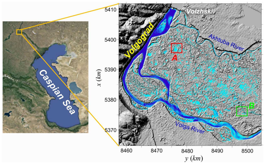
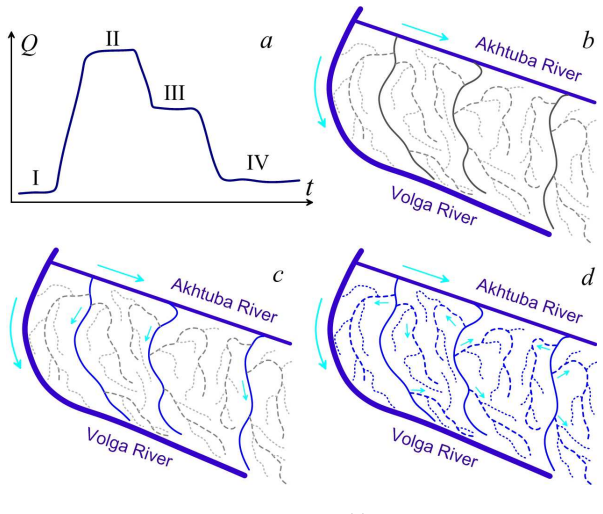
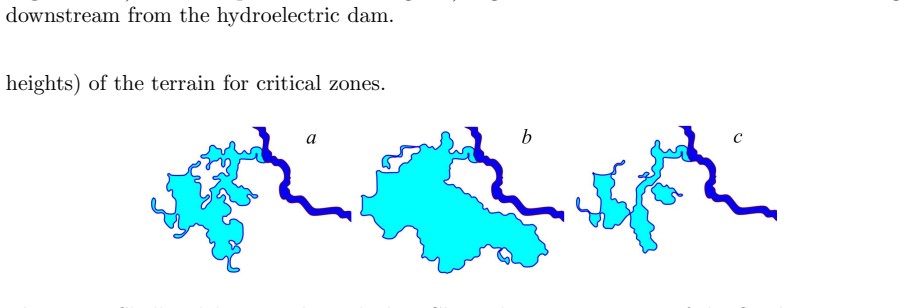
On the authors' own terms, the central discovery is that the moving coastlines of the many small reservoirs that form on the floodplain during spring flooding are a high-accuracy, low-cost source of elevation data: because each coastline coincides with a height contour, a short sequence of coastlines from the rising and falling flood yields a dense family of contour lines in the most hydrologically critical zones. Combining these coastline contours with embedded riverbed soundings and channel data, then smoothing the result with an iterative diffusion-type correction and flagging artifacts through morphostructural curvature analysis, produces a digital elevation model that the authors claim is significantly better than the base SRTM model. The hydrodynamic simulation of the same flood then serves as an independent check, because discrepancies between the modeled and observed flood extent are interpreted as remaining DEM errors to be corrected in the next iteration.

Load-bearing premise

The whole correction loop rests on the assumption that every observed waterline is a perfectly horizontal elevation contour, so any wind setup, water-surface slope, or vegetation bias makes the assigned height wrong.

Editorial extensions

If this is right

A corrected DEM for the Volga-Akhtuba floodplain can be produced and updated from flood imagery without new land surveys.
Digitized coastlines from UAV or satellite images become a routine source of elevation control for flat, seasonally flooded terrain.
Hydrodynamic flood simulations can double as DEM quality checks, since systematic mismatches with observed flood extent point to terrain errors.
Repeated flood events allow continuous updating of the DEM as erosion, sedimentation, and engineering works reshape the floodplain.

Reading between the lines

Editorial extensions of the paper, not claims the author makes directly.

I would expect the same coastline-as-contour procedure to transfer to other seasonal floodplains, deltas, and wetlands, with accuracy limited by how close the water surface is to perfectly horizontal.
A cheap controlled test would be to compare a DEM corrected only from publicly available satellite waterline time series against a lidar reference DEM in a small floodplain; the paper does not report such an independent accuracy assessment.
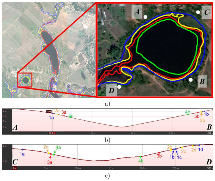
The waterline mismatches of 0.5-1 m on opposite slopes of the same reservoir, which the authors use to motivate correction, also set a practical floor on the vertical accuracy this method can promise unless wind setup and water-surface gradients are explicitly modeled.

Share X Bluesky LinkedIn Reddit HN

Signed reviews

No signed human review yet.

Editorial analysis

A structured set of objections, weighed in public.

Desk editor's note, referee report, and a circularity audit.

Desk Editor's Note

read the letter

Two things to know. The paper describes an iterative workflow for improving a floodplain DEM by fusing SRTM, river depth charts, satellite/UAV-derived waterlines of transient flood reservoirs, morphostructural analysis, and shallow-water hydrodynamic simulation. The new bit is using moving coastlines of seasonal lakes and eriks as elevation contours. That is a legitimate source of local topographic data in a data-sparse floodplain. The paper is clearly written, the equations are standard, and the integration logic is easy to follow.

What it does well: the pipeline is sensible and each ingredient is established. The diffusion-based interpolation for sparse depth points is standard. The morphostructural curvature and tilt screens are appropriate. The waterline observations are external to the DEM, so the main updates have independent grounding. The citation pattern is also fine; the self-citations point to the group's own shallow-water code, which is legitimate.

The soft spot is load-bearing: the assumption, stated in the Introduction and in Section 2.3, that each coastline coincides with a height contour 'with very high accuracy.' That holds only if the water surface is exactly level at every time. Flowing eriks and channels have a hydraulic gradient, and wind setup can tilt even small lakes by centimeters. The paper's own Figure 4 shows up to a meter of DEM scatter along a single coastline; the authors attribute all of it to DEM error, but a tilted water surface explains the same data. If the waterline is not horizontal, assigning one water level to all its points injects error of the same order as the claimed improvement.

The hydrodynamic verification in Section 2.4 is partly circular: the model runs on the DEM being tested, and every mismatch with observed flooding is attributed to DEM error. Without separately bounding model error (friction, boundary conditions, channel connectivity), that mismatch proves nothing about the DEM. There is no independent validation: no LiDAR, no RTK-GPS transects, no error bars, no quantitative before/after comparison. So the central claim that the procedure 'significantly improves' the DEM is not established.

This is a real flaw but a fixable one. The concept is not outlandish and the components are sound. The paper needs a validation section against independent high-accuracy terrain data on a small test area, plus a sensitivity analysis that allows water-surface slope per waterline.

Who this is for: researchers working on DEM refinement in floodplains and modelers who use hydrodynamic checks to audit topography. It deserves a serious referee; any acceptance should be conditioned on validation. I would not cite it as evidence of improvement until that validation appears, but I would read a revised version.

Referee Report

3 major / 5 minor

Summary. The paper describes an iterative procedure for constructing a digital elevation model (DEM) of the northern Volga-Akhtuba floodplain. The base data are SRTM elevations, refined with satellite imagery, GPS measurements, river depth soundings, and digitized coastlines of transient flood reservoirs. The key methodological idea is that observed coastlines of small lakes and eriks at different flood stages provide contour lines of elevation, which are assimilated into the DEM using a diffusion-based iterative scheme. The refined DEM is then checked through morphostructural analysis and shallow-water hydrodynamic simulations of spring flooding. The paper claims that this procedure can significantly improve DEM quality, but it provides no independent quantitative validation of that claim.

Significance. The proposed workflow is potentially valuable for floodplain DEM construction in data-sparse regions, because it exploits routinely observable waterline dynamics as elevation constraints at no additional field-survey cost. The diffusion-based interpolation in Eq. (4) is a standard and reasonable tool for assimilating sparse point data, and the use of hydrodynamic simulation as a plausibility check is a useful engineering idea. However, the central claim of 'significant improvement' is not supported by any error statistics, independent ground-control comparison, or uncertainty analysis. The paper also does not provide code or data, so the procedure cannot be reproduced from the text alone. If the required validation is added, the method could be a useful contribution to floodplain DEM construction; as it stands, the paper is a workflow description rather than a validated method.

major comments (3)

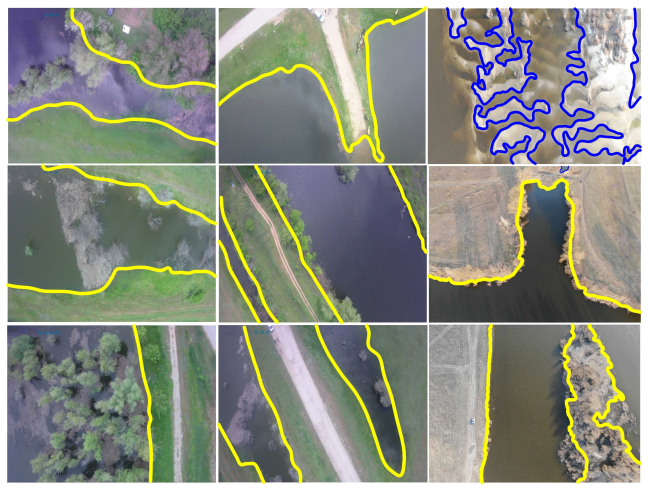
[Section 2.2, Eq. (4); Section 2.3] The load-bearing assumption that every digitized waterline is a horizontal elevation contour is stated in the Introduction and Section 2.3 but never quantitatively justified. Figure 4 shows that the same coastline intersects the AB and CD profiles at elevations differing by 0.5 m and 1 m in the current DEM; the authors attribute this entirely to DEM error, but a tilted water surface from wind setup or hydraulic gradients would produce the same discrepancy. If a waterline is not horizontal, assigning a single elevation value to all points along it in the assimilation step (Eq. (4)) introduces a systematic error of the same order as the claimed improvement. The authors should test the horizontal-contour assumption with independent water-level measurements along a waterline, or at minimum quantify the expected water-surface slope.
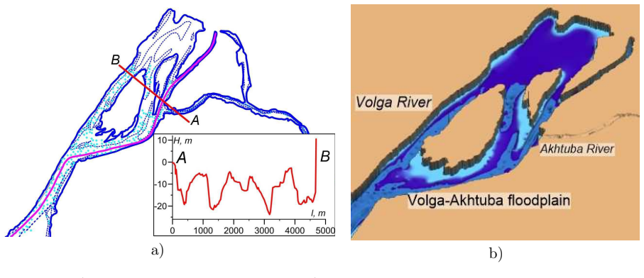
[Section 2.4] The hydrodynamic verification is not independent: the shallow-water model is run on the same DEM being refined, and the simulated flooded areas are compared with the observed waterlines that were already used as constraints in Section 2.2. Section 2.4 attributes every mismatch to DEM error, but no uncertainty analysis for the hydrodynamic model (friction coefficients, inflow hydrograph, boundary conditions, grid resolution) is provided. Without such analysis, the verification loop cannot separate DEM-induced misfit from model-induced misfit. The authors need to separate these contributions, for example by using independent high-accuracy elevation data (LiDAR, RTK-GPS transects) or by performing a formal model-uncertainty quantification.
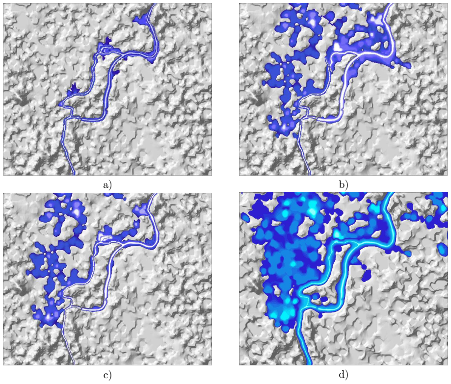
[Abstract; Section 2.1; Section 3] The central claim that the procedure can 'significantly improve the quality of the DEM' is not supported by any quantitative accuracy assessment. The paper reports no RMSE, mean absolute error, or any before/after statistics for the refined DEM, and there is no comparison with independent ground control points. Figures 7 and 9 are qualitative and show simulated flood patterns or visual DEM refinements, not measured terrain accuracy. To support the central claim, the authors should report quantitative error metrics for the initial SRTM-based DEM and for the final refined DEM against independent elevation observations, for example RMSE over RTK-GPS transects or LiDAR data.

minor comments (5)

[Section 2.2, Eq. (4)] The iterative diffusion scheme in Eq. (4) introduces a parameter alpha, but the paper gives no stopping criterion or method for choosing alpha; the statement that converging iterations yield Poisson's equation needs a derivation or reference. This information is necessary for reproducibility.
[Section 2.1, step 5] The morphostructural artifact detection in step 5 of Section 2.1 refers to 'areas with artifacts' but does not specify threshold values for the tilt angle s or the curvatures kt and ks; the procedure is therefore not fully reproducible.
[Figure 4] Figure 4 lacks a scale bar and clear annotation of the AB and CD profiles, so the reader cannot independently verify the quoted 0.5 m and 1 m elevation differences along the same coastline.
[General] There are several typographical and spacing errors in the text (e.g., 'carr ied out' in the Abstract, 'interﬂuve', and inconsistent notation for the successive DEM matrices b[1], b[2], b[3] versus b^p in Eq. (4)); these should be corrected.
[Section 2.1, item 2] The paper states that vectorized channel systems are 'introduced into the DEM matrix' but does not explain how the channel polygons are converted into elevation changes (e.g., by lowering grid nodes or carving a hydraulic profile); a short description of this step would improve clarity.

Circularity Check

1 steps flagged · score 6.0 of 10

DEM construction uses observed coastlines as constraints, then 'verifies' the DEM by comparing a hydrodynamic simulation against those same coastlines, making the claimed improvement partly circular.

fitted input called prediction [Section 2.4 and Fig. 9 caption; compare Sections 2.1(4) and 2.3]
"Comparison of simulation results with observational data is a powerful tool for updating the DEM ... By identifying the shortcomings of the DEM, we provide flooding in the model for the nearest areas in accordance with the observations."

The observed coastlines are first used as elevation constraints: Section 2.3 states that 'Measuring the position of coastline at different points in time can help us determine an additional set of contour lines (isolines of heights) of the terrain for critical zones,' and Section 2.1(4) says the refined matrix is 'the result of binding these isolines to heights.' The hydrodynamic model is then run on that same DEM and its output is compared with the very same coastline observations, with any mismatch attributed to DEM error. Because those observations were already assimilated into the DEM, agreement between modeled flooding and the observed coastlines is partly guaranteed by construction; using such agreement as independent verification of DEM quality is circular.

full rationale

The paper's core DEM update is grounded in external observational data (SRTM, satellite images, GPS, depth measurements, and digitized coastlines), so the construction step is not circular by itself. The circularity appears in the verification step: the same coastline observations that are used to impose elevation contours are later used to check the hydrodynamic simulation, and mismatches are always attributed to the DEM rather than to model physics or boundary conditions. This makes the claimed verification a fitted-input check rather than an independent test. The assumption that coastlines are horizontal contours is physically questionable, but that is a correctness risk, not a circularity, under the stated rules. The self-citations for the shallow-water solver are code references with independent computational content and do not by themselves raise the circularity score. Overall, the central claim of improved DEM retains independent data content, but the verification loop reduces to the input observations, giving a partial circularity score of 6.

Assumptions & free parameters 3 free parameters · 5 assumptions · 0 invented entities

The central claim rests on the external waterline data and on the assumption that model misfit is DEM error. No new physical entities are introduced. The main free parameters are the diffusion coefficient alpha, the interpolation grid step, and the morphometric thresholds, none of which are specified numerically.

free parameters (3)

alpha (diffusion iteration parameter)
Controls the convergence and smoothing in the iterative riverbed interpolation (Eq. 4); no value is reported, and the result depends on this hand-chosen parameter.
Interpolation grid step Delta x = 15 m, 10 m, 5 m
The SRTM matrix is resampled to these steps using weighted-averaging interpolation in 16 directions; the choice is discretionary and affects the spatial detail of the basic DEM.
Morphometric artifact thresholds
Morphostructural parameters (curvatures, tilt angles) are used to identify DEM artifacts, but threshold values for flagging errors are not specified.

assumptions (5)

domain assumption Observed coastlines are horizontal elevation contours with high accuracy.
Section 2.3 and Section 1 state that the coastline coincides with the height contour with very high accuracy; this is needed to convert observed waterlines into elevation constraints.
domain assumption The shallow-water model adequately represents floodplain hydrodynamics.
Section 2.4 uses a shallow-water numerical model to simulate flooding and to update the DEM; the approach assumes this model captures the relevant flow physics.
domain assumption SRTM data and the resampling procedure provide a reliable baseline.
Section 2.1 uses SRTM elevation data as the initial matrix and assumes that resampling and weighted interpolation preserve or improve the useful topographic signal.
domain assumption Simulation-observation mismatches can be attributed to DEM errors.
The procedure assumes that discrepancies between simulated and observed flooding can be corrected by editing the DEM; this is the circularity-prone premise in Section 2.4.
standard math The iterative diffusion formula converges to a Poisson equation solution.
The iterative formula (4) is stated to converge to the solution of Poisson's equation, relying on standard finite-difference theory.

how reviews work

0 comments

Cite this review

Pith. "Pith review of Creation of digital elevation models for river floodplains." pith.science (2026). https://pith.science/paper/DYEEHPPT

@misc{pith2026190809005,
  author       = {Pith},
  title        = {Pith review of: Creation of digital elevation models for river floodplains},
  year         = {2026},
  howpublished = {\url{https://pith.science/paper/DYEEHPPT}},
  note         = {Machine review of arXiv:1908.09005}
}

read the original abstract

A procedure for constructing a digital elevation model (DEM) of the northern part of the Volga-Akhtuba interfluve is described. The basis of our DEM is the elevation matrix of Shuttle Radar Topography Mission (SRTM) for which we carried out the refinement and updating of spatial data using satellite imagery, GPS data, depth measurements of the River Volga and River Akhtuba stream beds. The most important source of high-altitude data for the Volga-Akhtuba floodplain (VAF) can be the results of observations of the coastlines dynamics of small reservoirs (lakes, eriks, small channels) arising in the process of spring flooding and disappearing during low-flow periods. A set of digitized coastlines at different times of flooding can significantly improve the quality of the DEM. The method of constructing a digital elevation model includes an iterative procedure that uses the results of morphostructural analysis of the DEM and the numerical hydrodynamic simulations of the VAF flooding based on the shallow water model.

Figures

Figures reproduced from arXiv: 1908.09005 by the authors.

**Figure 1.** The northern part of the Volga-Ahtuba floodplain. A quality DEM is a critical component for all these tasks [13]. The terrain is a major physical factor that influences the dynamics of water. Unfortunately, the accuracy of best topographic maps is not high enough for numerical simulations. In addition, new problems appear on small spatial scales, and they are associated with changes in the surface of the relief caus… view at source ↗

**Figure 2.** Stages and sequence of DEM creation. of small reservoirs during the spring flood. These local DEMs are high-resolution data for the most critical areas in terms of hydrology as a part of global DEM for the northern territory of the Volga-Akhtuba floodplain ( [PITH_FULL_IMAGE:figures/full_fig_p003_2.png] view at source ↗

**Figure 3.** a — Typical dependence of discharge Q(t). b, c, d — The hierarchical structure of the hydrological system in the VAF at different stages of flooding. Volga ( [PITH_FULL_IMAGE:figures/full_fig_p004_3.png] view at source ↗

Figures from the paper (6 more)

**Figure 4.** Figure 4: The position of coastlines at different points in time for small bodies of water near the village Zonal’nyj. ( [PITH_FULL_IMAGE:figures/full_fig_p005_4.png]

**Figure 5.** Figure 5: The vectorization of water bodies images with UAV. The colored lines show the boundaries of the reservoirs. model. The morphostructural analysis of the DEM allows simple means to detect possible errors and promptly correct them, refining the hydrological network [20, 2…

**Figure 6.** Figure 6: a) The general structure of the VAF flooding is based on the results of our numerical hydrodynamic modeling. b) The distribution of water for the specified area of the frame. c) The distribution of the morphometric index ks for the same zone. We used an iterative proce…

**Figure 7.** Figure 7: a) Vector map of the River Volga. b) Digital elevation model of riverbed of the Volga downstream from the hydroelectric dam. heights) of the terrain for critical zones [PITH_FULL_IMAGE:figures/full_fig_p008_7.png]

**Figure 8.** Figure 8: Shallow lake near the Bulgakov Channel at various stagesof the flooding in 2014 is shown: a) start the flooding (May 6), b) maximum the flooding (May 8), c) the dissipation of the reservoir (May 18). 2.4. Verification based on the results of hydrodynamic simulations […

**Figure 9.** Figure 9: Results of local DEM refinement for the small river valley using hydrodynamic simulations. By identifying the shortcomings of the DEM, we provide flooding in the model for the nearest areas in accordance with the observations. procedure for creating the DEM for special…

Discussion (0). Continue with ORCID to comment.

Reference graph

Works this paper leans on

23 extracted references · 23 canonical work pages

[1]

Engineering 5 78708

Khrapov S S, Pisarev A V, Kobelev I A, Zhumaliev A G, Agafon nikova E O, Losev, A G and Khoperskov A V 2013 Advances in Mech. Engineering 5 78708

work page 2013
[2]

Informatics 8 627–638

Madadi M R, Azamathulla H M and Yakhkeshi M 2015 Earth Sci. Informatics 8 627–638

work page 2015
[3]

of the South Ural State Univ., Ser.: Mathem

Agafonnikova E O, Klikunova A Y and Khoperskov A V 2017 Bul. of the South Ural State Univ., Ser.: Mathem. Modelling, Program. and Comp. Software 10 148-55

work page 2017
[4]

5(4) 807–831

Jafary P, Sarab A Aand Tehrani N A 2018 Environmental Processes-an International J. 5(4) 807–831

work page 2018
[5]

Ermolaev O P, Mal’tsev K A and Ivanov M A 2014 Geography and Natural Resources 35(3) 222–228

work page 2014
[6]

Optics 42 695–703

Efremova O A, Kunakov Yu N, Pavlov S V and Sultanov A K 2018 Comp. Optics 42 695–703

work page 2018
[7]

and Inform

Voronin A, Isaeva I, Khoperskov A and Grebenuk S 2017 Communications in Comp. and Inform. Sci. 754 419–429

work page 2017
[8]

Optics 42(6) 1035–45

Boori M S, Paringer R, Choudhary K and Kupriyanov A 2018 Comp. Optics 42(6) 1035–45

work page 2018

Show all 23 references

[9]

116 64–76

Keenan P B and Jankowski P 2019 Decision Support Syst. 116 64–76

2019
[10]

Jonoski A and Seid A H 2016 Decision support in water resources planning and managemen t: the Nile basin decision support system Real-World Decision Support Syste ms (Cham: Springer) pp 199–222

2016
[11]

Grima N, Singh S J and Smetschka B 2017 Land use policy 67 73–85

2017
[12]

Modern Transportation 25 59–73

Bagloee S A, Tavana M, Di Caprio D, Asadi M and Heshmati M 2 017J. Modern Transportation 25 59–73
[13]

Satge F, Bonnet M P, Timouk F, Calmant S, Pillco R, Molina J, Lavado-Casimiro W, Arsen A, Cretaux J F and Garnier J 2015 Int. J. of Remote Sensing 36(2) 465–488

2015
[14]

Ahmed M F, Rogers J D and Ismail E H 2014 Europ. J. of Remote Sensing 47 343–373

2014
[15]

Reichenbach P, Rossi M, Malamud B D, Mihir M and Guzzetti F 2018 Earth-Science Reviews 180 60–91

2018
[16]

and Math

Sidoryakina V V and Sukhinov A I 2017 Computational Math. and Math. Phys. 57(6) 978–994

2017
[17]

Nikiforov S L, Sorokhtin N O, Lobkovsky L I and Koshel S M 2 018 Oceanology 58(2) 266–272
[18]

Optics 42(6) 1008–14

Michaelsen E 2018 Comp. Optics 42(6) 1008–14

2018
[19]

Optics 41(4) 564–572

Myasnikov E V 2017 Comp. Optics 41(4) 564–572

2017
[20]

& geosciences 59 116–123

Rueda A, Noguera J M and Martinez-Cruz C 2013 Comp. & geosciences 59 116–123

2013
[21]

Elmahdy S I 2015 Applied Geomatics 7(1) 1–11

2015
[22]

2018 A Numerical Simulation of the Shallow Water Flow ona Complex Topography Numerical Simulations in Engineering and Scien ce ed by Srinivasa Rao (InTechOpen) pp 237–254

Khoperskov A and Khrapov S. 2018 A Numerical Simulation of the Shallow Water Flow ona Complex Topography Numerical Simulations in Engineering and Scien ce ed by Srinivasa Rao (InTechOpen) pp 237–254

2018
[23]

and Inform

Dyakonova T A, Khoperskov A V and Khrapov S S 2016 Communications in Comp. and Inform. Sci. 687 132-145

2016

Pith tools

Reviewed August 14, 2026 · model on record in the stance chip above.

[1] [1]

Engineering 5 78708

Khrapov S S, Pisarev A V, Kobelev I A, Zhumaliev A G, Agafon nikova E O, Losev, A G and Khoperskov A V 2013 Advances in Mech. Engineering 5 78708

work page 2013

[2] [2]

Informatics 8 627–638

Madadi M R, Azamathulla H M and Yakhkeshi M 2015 Earth Sci. Informatics 8 627–638

work page 2015

[3] [3]

of the South Ural State Univ., Ser.: Mathem

Agafonnikova E O, Klikunova A Y and Khoperskov A V 2017 Bul. of the South Ural State Univ., Ser.: Mathem. Modelling, Program. and Comp. Software 10 148-55

work page 2017

[4] [4]

5(4) 807–831

Jafary P, Sarab A Aand Tehrani N A 2018 Environmental Processes-an International J. 5(4) 807–831

work page 2018

[5] [5]

Ermolaev O P, Mal’tsev K A and Ivanov M A 2014 Geography and Natural Resources 35(3) 222–228

work page 2014

[6] [6]

Optics 42 695–703

Efremova O A, Kunakov Yu N, Pavlov S V and Sultanov A K 2018 Comp. Optics 42 695–703

work page 2018

[7] [7]

and Inform

Voronin A, Isaeva I, Khoperskov A and Grebenuk S 2017 Communications in Comp. and Inform. Sci. 754 419–429

work page 2017

[8] [8]

Optics 42(6) 1035–45

Boori M S, Paringer R, Choudhary K and Kupriyanov A 2018 Comp. Optics 42(6) 1035–45

work page 2018