REVIEW 3 major objections 5 minor 14 references
Fundamentals of Drone Cellular Network Analysis under Random Waypoint Mobility Model
T0 review · 3 major / 5 minor · reviewed 2026-08-14 · deepseek-v4-flash
Pith's one-line read Random waypoint mobility preserves the Poisson structure of drone interference, making the time-dependent average user rate a closed-form integral.
desk verdict A genuine first-principles stochastic-geometry model for mobile drone networks, whose headline result rests on an unverified load-bearing simplification in Lemma 2 and an unquantified approximation. read the letter →
The pith
A machine-rendered reading of the paper's core claim, the machinery that carries it, and where it could break.
The reading
What carries the argument
Two mechanisms carry the argument. First, the displacement theorem (Lemma 1): if each point of a Poisson point process is displaced independently with an identical displacement distribution, the displaced points again form a Poisson point process with the same intensity, which is why the moving drone network never loses its Poisson character. Second, a closed-form approximation for the net displacement $Z_n$ of a drone after $n$ flights: the paper uses the exact Dirac and arcsine forms for $n=1,2$ and a truncated Rayleigh distribution for $n \geq 3$ (eq. (10)). This displacement distribution is inserted into the geometry of Lemma 2, which converts the time-varying exclusion zone and the random excursions of interferers into the explicit density $\lambda(t; u_x, u_0)$; that density is the object whose integral gives the average rate.
What would settle it
Simulate the exact simplified RWP process with fixed flight length $s$, hover time $w$, speed $v$, and initial Poisson density $\lambda_0$; for a range of times $t$ covering the first several flights, measure the empirical density of interfering drones around a typical user with nearest-neighbor association and compare it with the density from Lemma 2 built on eq. (10). A mismatch larger than the simulation error at early or intermediate times would mean the truncated-Rayleigh assumption is not good enough and the rate formulas in Theorem 1 are quantitatively wrong.
Extended reading notes
Core claim
The paper's central claim is that Poisson tractability survives drone mobility. Starting from drone base stations whose ground projections form a homogeneous Poisson point process of density $\lambda_0$, and letting every drone move under the simplified RWP model (hover, random direction, fixed flight distance, repeat), the interference field seen by a typical user under nearest-neighbor association is again an inhomogeneous Poisson point process. For the UE-independent model the density is static, equal to $\lambda_0$ everywhere except an exclusion zone around the serving drone. For the UE-dependent model, where the serving drone flies toward the user and hovers above it, the density is time-dependent and is given explicitly in Lemma 2 through the displacement distribution $L(t)$. Feeding this density into the probability generating functional of the Poisson point process yields the average rate at time $t$ (Theorem 1), so the whole performance analysis reduces to one time-varying density function.
Load-bearing premise
The whole calculation depends on treating the total distance a drone has wandered from its starting point after three or more random-direction flights as a bell-shaped distribution cut off at the maximum possible travel distance; the paper offers no error bound for that approximation, so if it loses accuracy at some flight counts, speeds, or hover times, the interference density and the rate expressions inherit the error.
Editorial extensions
If this is right
- In the UE-independent model the average rate is constant in time, because the interference density has the same distribution at every instant even while every drone keeps moving.
- In the UE-dependent model the average rate grows as the serving drone approaches the user and saturates as the interference field becomes homogeneous in the limit of large time.
- Raising the drone operating height lowers the average rate, through the extra path loss on both the serving and interfering links.
- The straight-line drone mobility model used by standardization bodies is covered as a special case, so the closed-form expressions apply to that benchmark without further derivation.
- The explicit time-varying interference density lets operators compare hover-and-turn missions against straight-line missions across time, replacing per-parameter simulation with evaluation of two integrals.
Reading between the lines
- A straightforward extension would replace the fixed flight distance and hover time with random ones; Lemma 2's geometric template would survive as long as displacements stay independent, but the displacement distribution would need a new approximate form.
- The Laplace-transform step in the proof already contains the coverage probability at any SIR threshold, so the same density yields coverage curves in addition to the average rate reported here.
- A testable prediction from the figures is that the rate gap between the UE-dependent and UE-independent models widens with time and narrows at higher flight heights; this can be checked directly from the closed-form integrals without simulation.
Signed reviews
Editorial analysis
A structured set of objections, weighed in public.
Referee Report
Summary. This paper studies the downlink of a drone cellular network in which drone base stations (DBSs) are initially distributed as a homogeneous Poisson point process (PPP) and move according to a simplified random waypoint (SRWP) mobility model. The typical ground user connects to the nearest DBS. Two service models are considered: a UE-independent model (UIM), in which the serving DBS also follows SRWP, and a UE-dependent model (UDM), in which the serving DBS moves to hover above the user. Using the displacement theorem, the authors characterize the time-varying interference field as an inhomogeneous PPP for both models and derive average rate expressions in Theorem 1. The central technical result is Lemma 2, which gives the UDM interference density in terms of the displacement distribution of an SRWP drone, built on the distributional properties of the net displacement after n flights.
Significance. The paper proposes a novel and timely analysis: to my knowledge, it is the first stochastic-geometry treatment of drone mobility under a random waypoint model on an infinite plane. The displacement-theorem perspective is elegant and yields closed-form rate expressions that are useful for system design, and the separation into UIM and UDM cleanly captures the trade-off between serving-DBS tracking and interference dynamics. The paper also carefully handles the nearest-neighbor association with a moving serving DBS. However, the central UDM density rests on an explicitly omitted integration step and on a finite-n approximation without error bounds, so the quantitative claims are not yet fully supported.
major comments (3)
- [Section III, Lemma 2, Appendix A] The proof of Lemma 2 stops at the double integral in Eq. (18) and states that "Simplifying the last step requires careful integrations and the details are omitted here for brevity." This omitted reduction is load-bearing: the closed-form density in Eqs. (3)-(4) is the foundation for the rate expression in Theorem 1, and without it a reader cannot verify the correctness of the central result. Please provide the full derivation or an independent verification (e.g., a symbolic-computation script), and in any case add a more extensive numerical check of the density expression beyond the four curves in Fig. 2.
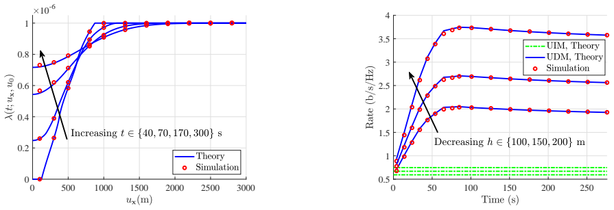
- [Section III, Eq. (10)] The truncated Rayleigh approximation for the distribution of Z_n is used for all n≥3 without an error bound. The CLT justification in Lemma 4 is asymptotic, and n=3 is far from the asymptotic regime. The simulation in Fig. 2 uses t=40, 70, 170, 300 s, which for the stated parameters (s=250 m, v=45 km/h, w=5 s) correspond to n=1, 2, 6, 11, thus skipping the n=3-5 regime where the approximation is most likely to be inaccurate. Since the distribution of L_n(t) feeds directly into Lemma 2 and hence into Theorem 1, the quantitative validity of the rate formula is not established for all times and parameter values. Please add an error analysis or simulations that include n=3-5 and vary s, w, v, and h.
- [Section III, Remark 1] Remark 1 states that Φ_n has a "symmetric triangular distribution" and then concludes "we have Φ_n∼U[0,2π)." This is contradictory as written: a triangular distribution is not uniform. While the wrapped difference of two independent uniform [0,2π) variables is indeed uniform, the explanation must be corrected because Eq. (11) relies on the uniform distribution of cos(Φ_n) to evaluate the probability integral. The current text could mislead a reader into thinking the derivation is flawed.
minor comments (5)
- [Eq. (13)] The display of Eq. (13) appears to be missing the differential dγ in the outer integral; the proof text correctly ends with "du0 dγ." Please add the missing differential.
- [Abstract and Introduction] The claim of being the "first work that analyzes the performance of a mobile drone network in which the drones follow an RWP mobility model on an infinite plane" is slightly overstated given Ref. [12] treats random 3D mobile UAV networks with RWP. Please qualify the novelty (infinite plane, PPP initial condition, average rate metric, etc.).
- [Section III, Lemma 3] The derivation of fΨn(ψn) first gives 1/π on [-π/2,π/2) due to the range of the tan^{-1} function and then asserts that the full range [-π,π) yields 1/(2π). This is not rigorous as written; a short argument using the rotational symmetry of the sum of isotropic vectors would be cleaner and would avoid the apparent discontinuity.
- [Fig. 2 and Numerical Results] Please include the simulation parameters and the number of Monte Carlo runs used in Fig. 2, and clarify which curves are analytic and which are simulated. The caption currently says "accuracy of our approximations is evident" without specifying the simulation details.
- [Index Terms] There is a typo in the index terms line: "Index Terms —Drone network" should have a space after the em dash.
Circularity Check
No circularity: the rate and density derivations are self-contained given standard displacement theorem and CLT results; remaining issues are rigor gaps, not circularity.
full rationale
The paper's central claims are that under the SRWP mobility model the interfering DBSs form an inhomogeneous PPP with density given by Lemma 2 (eqs. (3)-(4)), and that the average rate in Theorem 1 follows from the PGFL of that PPP. The derivation chain is: standard displacement theorem (Ref. [14], an external textbook), the SRWP geometry in eqs. (5)-(7), a CLT-based truncated Rayleigh approximation for Z_n in eq. (10), and the integral manipulations in Appendix A. No parameter is fitted to simulation data or to the output quantities; the truncated Rayleigh approximation is an explicit modeling choice, and Fig. 2 validates rather than calibrates it. The only self-citation is [6] (Chetlur and Dhillon) in a related-work paragraph, and it is not load-bearing. The appendix does omit the algebraic simplification connecting the double integral (18) to the closed-form density in (3)-(4), and eq. (10) is used for n >= 3 without an error bound; these are correctness/completeness concerns, but they are not circular because the claimed formulas are not assumed as inputs anywhere. No equation is defined in terms of the quantity it is supposed to predict, and no fitted input is renamed as a prediction. Hence the circularity burden is low and the honest finding is no significant circularity.
Assumptions & free parameters
assumptions (8)
- domain assumption Initial drone locations form a homogeneous PPP with density lambda0.
- domain assumption UE process is an independent PPP.
- domain assumption Rayleigh fading with unit mean.
- domain assumption Drone trajectories are independent across drones and follow SRWP.
- standard math Displacement theorem: independent iid displacement of a PPP yields a PPP.
- standard math Central limit theorem for sums of iid random vectors.
- ad hoc to paper For n>=3 flights, Z_n is approximated by a truncated Rayleigh distribution (eq 10).
- domain assumption In UDM, the serving DBS always remains the nearest DBS, so the exclusion zone radius u0(t) is valid.
Cite this review
Pith. "Pith review of Fundamentals of Drone Cellular Network Analysis under Random Waypoint Mobility Model." pith.science (2026). https://pith.science/paper/MLW6OQUS
@misc{pith2026190809064,
  author       = {Pith},
  title        = {Pith review of: Fundamentals of Drone Cellular Network Analysis under Random Waypoint Mobility Model},
  year         = {2026},
  howpublished = {\url{https://pith.science/paper/MLW6OQUS}},
  note         = {Machine review of arXiv:1908.09064}
}
read the original abstract
In this paper, we present the first stochastic geometry-based performance analysis of a drone cellular network in which drone base stations (DBSs) are initially distributed based on a Poisson point process (PPP) and move according to a random waypoint (RWP) mobility model. The serving DBS for a typical user equipment (UE) on the ground is selected based on the nearest neighbor association policy. We further assume two service models for the serving DBS: (i) UE independent model (UIM), and (ii) UE dependent model (UDM). All the other DBSs are considered as interfering DBSs for the typical UE. We introduce a simplified RWP (SRWP) mobility model to describe the movement of interfering DBSs and characterize its key distributional properties that are required for our analysis. Building on these results, we analyze the interference field as seen by the typical UE for both the UIM and the UDM using displacement theorem, which forms the basis for characterizing the average rate at the typical UE as a function of time. To the best of our knowledge, this is the first work that analyzes the performance of a mobile drone network in which the drones follow an RWP mobility model on an infinite plane.
Figures


Reference graph
Works this paper leans on
-
[1]
Mobility increases the capacity of ad hoc wireless networks,
M. Grossglauser and D. N. C. Tse, “Mobility increases the capacity of ad hoc wireless networks,” IEEE/ACM Trans. Netw., vol. 10, no. 4, pp. 477–486, Aug. 2002
work page 2002
-
[2]
Stochastic properties of mobility models in mobile ad hoc networks,
S. Bandyopadhyay, E. J. Coyle, and T. Falck, “Stochastic properties of mobility models in mobile ad hoc networks,” IEEE Trans. Mobile Comput., vol. 6, no. 11, pp. 1218–1229, Nov. 2007
work page 2007
-
[3]
The node distribution of the random waypoint mobility model for wireless ad hoc networks,
C. Bettstetter, G. Resta, and P. Santi, “The node distribution of the random waypoint mobility model for wireless ad hoc networks,” IEEE Trans. Mobile Comput. , vol. 2, no. 3, pp. 257–269, July 2003
work page 2003
-
[4]
Wireless communications with un- manned aerial vehicles: Opportunities and challenges,
Y . Zeng, R. Zhang, and T. J. Lim, “Wireless communications with un- manned aerial vehicles: Opportunities and challenges,” IEEE Commun. Mag., vol. 54, no. 5, pp. 36–42, May 2016
work page 2016
-
[5]
A tutorial on UA Vs for wireless networks: Applications, challenges, and open problems,
M. Mozaffari, W. Saad, M. Bennis, Y . Nam, and M. Debbah, “A tutorial on UA Vs for wireless networks: Applications, challenges, and open problems,” IEEE Commun. Surveys Tut. , to appear
-
[6]
Downlink coverage analysis for a finite 3-D wireless network of unmanned aerial vehicles,
V . V . Chetlur and H. S. Dhillon, “Downlink coverage analysis for a finite 3-D wireless network of unmanned aerial vehicles,” IEEE Trans. Commun., vol. 65, no. 10, pp. 4543–4558, Oct. 2017
2017
-
[7]
X. Wang, H. Zhang, Y . Tian, and V . C. M. Leung, “Modeling and analysis of aerial base station-assisted cellular networks in finite areas under LoS and NLoS propagation,” IEEE Trans. Wireless Commun. , vol. 17, no. 10, pp. 6985–7000, Oct. 2018
work page 2018
-
[8]
Moving aerial base station networks: A stochastic geometry analysis and design perspective,
S. Enayati, H. Saeedi, H. Pishro-Nik, and H. Yanikomeroglu, “Moving aerial base station networks: A stochastic geometry analysis and design perspective,” IEEE Trans. Wireless Commun., vol. 18, no. 6, pp. 2977– 2988, June 2019
work page 2019
Show all 14 references
-
[9]
Capacity analysis of UA V communications: Cases of random trajectories,
X. Yuan et al. , “Capacity analysis of UA V communications: Cases of random trajectories,”IEEE Trans. Veh. Technol., vol. 67, no. 8, pp. 7564– 7576, Aug. 2018
2018
-
[10]
Fundamentals of mobility- aware performance characterization of cellular networks: A tutorial,
H. Tabassum, M. Salehi, and E. Hossain, “Fundamentals of mobility- aware performance characterization of cellular networks: A tutorial,” IEEE Commun. Surveys Tut. , to appear
-
[11]
Coverage probability of 3-D mobile UA V networks,
P. K. Sharma and D. I. Kim, “Coverage probability of 3-D mobile UA V networks,” IEEE Wireless Commun. Lett., vol. 8, no. 1, pp. 97–100, Feb. 2019
2019
-
[12]
Random 3D mobile UA V networks: Mobility modeling and coverage probability,
——, “Random 3D mobile UA V networks: Mobility modeling and coverage probability,” IEEE Trans. Wireless Commun. , vol. 18, no. 5, pp. 2527–2538, May 2019
2019
-
[13]
Enhanced LTE support for aerial vehicles,
3GPP, “Enhanced LTE support for aerial vehicles,” 3rd Generation Partnership Project (3GPP), Tech. Rep. 36.777, 01 2018, version 1.1.0
2018
-
[14]
Haenggi, Stochastic Geometry for Wireless Networks
M. Haenggi, Stochastic Geometry for Wireless Networks . Cambridge University Press, 2012
2012
Reviewed August 14, 2026 · model on record in the stance chip above.
Discussion (0). Continue with ORCID to comment.