REVIEW 2 major objections 5 minor 1 cited by
Optimal $\delta$-Correct Best-Arm Selection for Heavy-Tailed Distributions
T0 review · 2 major / 5 minor · reviewed 2026-08-14 · deepseek-v4-flash
Pith's one-line read A δ-correct algorithm for unbounded-support arms can match the sample-complexity lower bound when the algorithm knows a moment bound E f(|X|) ≤ B, and is provably impossible without such a restriction.
desk verdict Significant results and a real gap: the δ-correct algorithm's threshold C depends on the unknown arm distributions, so Theorem 10 is not yet a fully specified algorithm for L. read the letter →
The pith
A machine-rendered reading of the paper's core claim, the machinery that carries it, and where it could break.
The reading
What carries the argument
The load-bearing object is $KL_{\inf}(\eta,x)$, the minimum Kullback-Leibler divergence from an arm distribution $\eta$ to any distribution in $\mathcal{L}$ whose mean lies on the required side of $x$; it measures how hard it is to confuse $\eta$ with an alternative arm of mean $x$. This functional carries both halves of the argument: the lower bound $V(\mu)$ is a max-min over allocation proportions of sums of $KL_{\inf}$, and the algorithm's generalized likelihood-ratio stopping statistic is the same sum evaluated at empirical distributions. Theorem 12 gives a dual representation, $KL_{\inf}(\eta,x)=\max_{(\lambda_1,\lambda_2)\in R_2} E_\eta \log(1-(X-x)\lambda_1-(B-f(|X|))\lambda_2)$, a two-variable concave maximization over Lagrange multipliers for the mean and moment constraints. That makes the functional computable and yields exponential concentration inequalities for its empirical version; compactness of $\mathcal{L}$ in the Wasserstein metric plus Berge's maximum theorem then make the optimal proportions $t^*(\mu)$ and the value $V(\mu)$ continuous in the arm distributions, so the plug-in sampling rule converges to the oracle proportions.
What would settle it
Take a two-arm instance with Pareto distributions, set $f(y)=y^2$ and $B$ equal to the second moment of the better arm while the other arm has second moment $B+\varepsilon$, run AL1 with the declared $B$ for $\delta=10^{-3},10^{-6},10^{-8}$, and measure the empirical error frequency and $E_\mu(\tau_\delta)/\log(1/\delta)$; error above $\delta$ or a ratio that does not approach $1/V(\mu)$ would refute Theorem 10 on that instance.
Extended reading notes
Core claim
The paper's central claim is that a known moment-type bound is the right dividing line between tractable and intractable $\delta$-correct best-arm selection. On the intractable side, Theorem 3 shows that if the allowed class of distributions is KL right dense — meaning every arm distribution can be perturbed by arbitrarily small KL divergence into another distribution in the class with a larger mean — then under any $\delta$-correct algorithm $E_\mu N_k(\tau) = \infty$ for every non-best arm $k \ge 2$. On the tractable side, Theorem 10 shows that for the class $\mathcal{L} = \{\eta : E_\eta f(|X|) \le B\}$, algorithm AL1 with the stopping threshold $\beta(n,\delta) = \log(C n^\alpha / (\delta (\log n)^K (\log(1/\delta))^{2K+1}))$ and batch size $m = o(\log(1/\delta))$ is $\delta$-correct and satisfies $\limsup_{\delta\to 0} E_\mu(\tau_\delta)/\log(1/\delta) \le 1/V(\mu)$, where $V(\mu)$ is the value of the max-min lower-bound problem. In words, once the algorithm is handed a valid moment bound, it stops with error at most $\delta$ and its sample complexity reaches the lower bound to first order as $\delta$ shrinks.
Load-bearing premise
The load-bearing premise is that the algorithm is handed a correct pair $(f,B)$ that really bounds $E f(|X|)$ for every arm; if the bound is wrong, unknown, or the true distribution violates it, the $\delta$-correctness proof and the matching constant $V(\mu)$ no longer apply.
Editorial extensions
If this is right
- For any finite set of arms satisfying a known bound $E f(|X|) \le B$, AL1 gives first-order optimal sample complexity, roughly $\log(1/\delta)/V(\mu)$, while keeping the error probability at most $\delta$.
- Without such a bound, the problem is hopeless in expectation: every $\delta$-correct algorithm pulls every suboptimal arm infinitely often when the allowed class is KL right dense.
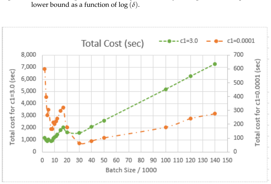
- Under the paper's cost model, the batch size minimizing total sampling-plus-computation cost is $\Theta(\log(1/\delta))$; this preserves $\delta$-correctness but loses the asymptotic optimality ratio, whereas $m = o(\log(1/\delta))$ preserves both.
- The theory reduces the previous exponential-family-only setting to a special case: when arms form a single-parameter exponential family, $KL_{\inf}$ collapses to ordinary KL divergence between exponential-family distributions.
- If bounded support is known in advance, the dual problem becomes one-dimensional, and the same algorithm simplifies while retaining $\delta$-correctness and asymptotic optimality.
Reading between the lines
- Estimating $(f,B)$ from early samples with a conservative confidence multiplier is a natural extension, but the paper does not analyse it; whether $\delta$-correctness survives with only a $\log\log(1/\delta)$ penalty is open.
- The KL right-density impossibility should transfer to $\delta$-correct selection of other unbounded functionals, such as quantiles or variances: without a known envelope constraint, the same transportation inequality forces infinite expected pulls.
- A practical reading of the batch-size analysis is that the user's ratio of sampling cost to computation cost determines whether to batch aggressively (cheap samples) or finely (expensive samples); making the batch size adapt online is left open.
- The dual representation of $KL_{\inf}$ is a reusable template for other constraint sets, e.g., known bounds on $E e^{\lambda X}$ or on variance, which would yield a family of $\delta$-correct algorithms beyond the class $\mathcal{L}$ studied here.
Signed reviews
Editorial analysis
A structured set of objections, weighed in public.
Referee Report
Summary. This paper studies δ-correct best-arm selection for K distributions with finite means. The authors prove an impossibility result (Theorem 3) for KL-right-dense unbounded-support classes, showing that any δ-correct algorithm must have infinite expected pulls on non-best arms. For the class L defined by a known bound B on E f(|X|) with f strictly increasing, convex, and superlinear, they formulate the max-min lower-bound problem, characterize its solution V(μ) and optimal proportions t*(μ) (Theorem 5), derive a dual representation of the KLinf functional (Theorem 12), prove concentration inequalities for empirical KLinf (Theorems 11 and 13), and propose the sampling algorithm AL1 with a generalized-likelihood-ratio stopping rule (Section 4). They claim that AL1 with threshold β(n,δ) = log(C n^α (log n)^K (log 1/δ)^{2K+1} / δ), with m = o(log(1/δ)), is δ-correct and satisfies limsup E_μ(τ_δ)/log(1/δ) ≤ 1/V(μ) (Theorem 10). The paper also discusses batch-size optimization and includes a numerical study with Pareto arms.
Significance. The negative result and the general moment-bound framework are valuable contributions that extend fixed-confidence best-arm theory beyond single-parameter exponential families and bounded-support settings. The dual representation of KLinf and the concentration inequalities are potentially reusable tools. The paper is also careful to include full proofs in the appendices and a numerical demonstration. However, the main algorithmic claim is currently tied to a threshold constant that is not computable from the stated problem data, and a continuity argument used in the proof of Theorem 5 is not justified as written. These are substantive issues that need to be repaired before the central contribution can be accepted.
major comments (2)
- [Section 4, Eq. (16) and Theorem 10] The constant C in the threshold β(n,δ) is defined only through inequality (16), whose left side contains the factor ∏_a e^{B̃_a}. As defined before Theorem 13 (and analogously before Theorem 11), B̃_a depends on the true distribution μ_a through E|X−m(μ_a)| and through the denominators f^{-1}(B)−m(μ_a) and B−f(|m(μ_a)|). Since AL1 must be run knowing only f, B, K, and δ, this C is not computable from the problem data. Moreover, B̃_a is unbounded over L: for f(y)=y² and B=1, the two-point distribution at 1−ε±√(2ε−ε²) lies in L with mean 1−ε and E X²=1, while the corresponding constant d_{a1} = c_{a1}/(2(f^{-1}(B)−m(μ_a))) is Ω(ε^{−1/2}) as ε→0. Hence the minimal C satisfying (16) diverges over L, so no single threshold of the form (10) can make AL1 δ-correct over all of L from the stated problem data alone. The authors must either supply an explicit distribution-free constant (possibly via a different concentration argument), replace the threshold with a data-dependent stopping rule, or clearly restrict the theorem to per-instance constants, in which case AL1 would no longer be a well-defined algorithm for unknown μ.
- [Appendix B.1, Lemma 4] The proof of Lemma 4 asserts without argument that KL(·,·) is continuous on the Wasserstein metric space (P(R), d_W). This is false: with f(y)=y² and B=1, take η = 0.5 δ_0 + 0.5 δ_1 and κ_n = 0.5 δ_{1/n} + 0.5 δ_1. Both are in L, d_W(η, κ_n)→0, but KL(η,κ_n)=∞ for every n. The subsequent use of Berge's maximum theorem to conclude continuity of KLinf(η,x), and through Theorem 5 the continuity of t*(μ), is therefore not justified. Since t* continuity underpins Lemma 14 and the sample-complexity proof, this continuity claim needs a direct proof (or a lower-semicontinuity argument adapted to the compact class L), not an appeal to the global continuity of KL.
minor comments (5)
- [Title/Abstract] The arXiv title emphasizes 'Heavy-Tailed Distributions' while the manuscript title on the first page is 'Optimal δ-Correct Best-Arm Selection for General Distributions'; please reconcile the titles with the actual scope of the class L.
- [Eq. (10)] The argument of the logarithm in (10) is ambiguous; please write it as log(C n^α (log n)^K (log(1/δ))^{2K+1} / δ) with clear parentheses.
- [Before Theorems 11 and 13] The notation B̃_a is used inconsistently: before Theorem 11 it is d1+d2, while before Theorem 13 the displayed definition says B̃_a = c_{a1}+c_{a2}. Please harmonize the notation so that it is unambiguous which quantity appears in the concentration bounds.
- [Section 5, numerical experiment] The text states that results are averaged over 20 independent experiments, but later says 'in all the 15 independent experiments'; please correct the inconsistent count.
- [Remark 7] The complexity claim for solving the max-min problem would benefit from a brief explanation of how interpolation error is controlled, since the empirical distributions are reused in the stopping rule.
Circularity Check
Theorem 10's threshold constant C is defined through µ-dependent constants in (16), so AL1's δ-correctness is obtained by allowing the stopping rule to depend on the unknown distributions.
-
self definitional
[Section 4, stopping rule (10), constants before Theorem 13, and inequality (16) in the proof of (12)]
"Let ca1 = Eµa(|X−x|), ca2 = Eµa(|B−f(|X|)|), da1 = ca1/(2(f−1(B)−m(µa))), and da2 = ca2/(2(B−f(|µa|))) be non-negative constants and let ˜Ba≜ca1+ca2. ... Further, choosing the constant C as: [inequality (16) containing ∏a e^{˜Ba}], proves that ∑∞l=1 P(El), and hence P(E) is bounded from above by δ."
The stopping threshold β(n,δ) in (10) contains C, and C is selected via (16) so that the union-bound error probability is at most δ. But the left side of (16) contains ∏a e^{B̃a}, where B̃a is defined just before Theorem 13 from the true, unknown arm distributions µa: it depends on E|X−m(µa)|, E|B−f(|X|)|, and the denominators f−1(B)−m(µa) and B−f(|m(µa)|). Thus the algorithm's threshold is specified only by feeding the unknown µ into the algorithm; the δ-correctness claim is not derived for a well-defined distribution-free algorithm. The dependence is not removable within the paper's argument: as m(µa) approaches f−1(B), the denominator f−1(B)−m(µa) tends to zero and B̃a can grow without bound, so no single C computed from f, B, δ, and K alone can satisfy (16) for the whole class L.
full rationale
Apart from the threshold-constant issue, the paper's derivation chain is largely self-contained. The lower-bound benchmark V(µ) is derived from the standard transportation inequality and a max-min optimization whose solution is proved here; the concentration inequalities for KLinf are proved from a dual representation that extends Honda--Takemura rather than being assumed; and the sample-complexity matching argument uses the empirical proportions and continuity properties developed in the paper. The self-citations (Glynn--Juneja 2004 for the max-min characterization analogy and Juneja--Krishnasamy 2019 for the plug-in sampling strategy) are not load-bearing: the present paper supplies its own proofs. The significant circular dependency is confined to the δ-correctness proof of Theorem 10, where the constant C in the stopping rule is chosen from the very arm distributions the algorithm is supposed not to know. That makes the central algorithmic claim partially circular by construction, even though the asymptotic optimality bound retains independent content.
Assumptions & free parameters
assumptions (4)
- domain assumption Transportation inequality (Eq. 2): for any δ-correct algorithm and any alternative ν, Σ_i E_μ N_i(τ) KL(μ_i, ν_i) ≥ ρ(δ, 1-δ).
- standard math Berge's Maximum Theorem, stated in Appendix A.1.
- standard math Classical exponential inequalities: Sanov's theorem, Chernoff bounds, and Azuma-Hoeffding inequality.
- domain assumption The distribution class L (Eq. 1) with known f and B and f(y)/y → ∞.
Cite this review
Pith. "Pith review of Optimal $\delta$-Correct Best-Arm Selection for Heavy-Tailed Distributions." pith.science (2026). https://pith.science/paper/UW3ZYWWU
@misc{pith2026190809094,
  author       = {Pith},
  title        = {Pith review of: Optimal $\delta$-Correct Best-Arm Selection for Heavy-Tailed Distributions},
  year         = {2026},
  howpublished = {\url{https://pith.science/paper/UW3ZYWWU}},
  note         = {Machine review of arXiv:1908.09094}
}
abstract
Given a finite set of unknown distributions or arms that can be sampled, we consider the problem of identifying the one with the maximum mean using a $\delta$-correct algorithm (an adaptive, sequential algorithm that restricts the probability of error to a specified $\delta$) that has minimum sample complexity. Lower bounds for $\delta$-correct algorithms are well known. $\delta$-correct algorithms that match the lower bound asymptotically as $\delta$ reduces to zero have been previously developed when arm distributions are restricted to a single parameter exponential family. In this paper, we first observe a negative result that some restrictions are essential, as otherwise, under a $\delta$-correct algorithm, distributions with unbounded support would require an infinite number of samples in expectation. We then propose a $\delta$-correct algorithm that matches the lower bound as $\delta$ reduces to zero under the mild restriction that a known bound on the expectation of $(1+\epsilon)^{th}$ moment of the underlying random variables exists, for $\epsilon > 0$. We also propose batch processing and identify near-optimal batch sizes to speed up the proposed algorithm substantially. The best-arm problem has many learning applications, including recommendation systems and product selection. It is also a well-studied classic problem in the simulation community.
Figures

Forward citations
Cited by 1 Pith paper
-
Decision-Centric Large Deviations for Data-Driven Capital Buffers in Ruin Models
A data-driven capital buffer for ruin models is safe only above a pointwise profile f*; the naive plug-in of the estimated adjustment coefficient misses the target exponential decay rate.
Reference graph
Works this paper leans on
-
[1]
for j∈{2, . . . ,K}. Note that c∗ ∈ [KLinf(µ1, m(µ1)), dj) for all j∈{2, . . . ,K}. Let d = minj dj. Then, c∗∈ [KLinf(µ1, m(µ1)), d)
-
[2]
For a fixed c∈ [0, d), and for each j∈{2, . . . ,K}, solve the following for yj = yj(c) (set y1(c) = 1) and let xj(c) for each j≥ 2 denote the corresponding minimizer: inf x∈[m(µj),m(µ1)] KLinf(µ1, x) + yj KLinf(µj, x) = c
-
[3]
Fix c = KLinf(µ1, m(µ1))
-
[4]
Output t∗ j = yj(c∗)/∑K i=1 yi(c∗) for all y∈{1, . . . ,K} and V(µ) = c∗t∗ 1. Appendix C. Proofs related to the sampling algorithm We first prove that at the end of each interval of length m, say l, the sampling algorithm ensures a minimum ( √ lm− 1) number of samples to each arm, i.e., Na(lm)≥ √ lm− 1. C.1 Proof of Lemma 8 The above is true for l = 1 as N...
work page 1969
-
[5]
Line search for c∗ in the interval [KLinf(µ1, m(µ1)), d), so that with yj(c∗) and the corresponding xj(c∗) computed using Step 2, the following holds: K ∑ j=2 KLinf(µ1, xj(c∗)) KLinf(µj, xj(c∗)) = 1
-
[7]
Henceforth, in our discussion, we consider only such rectangles. Lemma 28 For any ua∈ℜ , non-negative constants ˜Ba and rectangle Ga, P ( K⋂ a=1 { max λa∈Ga L(λa, m(µa), ˆµa(n))≥ ua,Cd a }) ≤ K ∏ a=1 e ˜Bae−taua. Proof Recall that Ga is a rectangle that intersects the regionRa
-
[8]
Letλa0 = ( λa 10, λa
-
[10]
Observe from (52) that max λa∈Ga Na(n)L(λa, m(µa), ˆµa)≤ Sa(n,λa0). Thus, P ( K⋂ a=1 { max λa∈Ga L(λa, m(µa), ˆµa(n))≥ ua,Cd a }) ≤ P ( K⋂ a=1 { Sa(n,λa0)≥ Na(n)ua,Cd a }) ≤ P 1 Cde { K ∑ a=1 θaSa(n,λa0) } ≥ e { K ∑ a=1 θaNa(n)ua } . Multiplying by exp{−Na(n)Λa(θa,λa0)} on both sides of the inequality in the above ex- pression, the probability of in...
Show all 12 references
-
[11]
generalized likelihood ratio
Substi- tuting this back into (55) and choosing θ = 1 for all a, we get the following desired upper bound: P ( K⋂ a=1 { max λ1∈Ga L(λa, m(µa), ˆµa(n))≥ ua,Cd a }) ≤ K ∏ a=1 e ˜Bae−taua. (56) Using the above result, we prove following inequality, which will assist in the proof ...
2002
-
[12]
To this end, Figure 1 plots the ratio of average number of samples needed by AL1 to stop, and the lower bound on this quantity, as a function of log (δ)
the lower bound on this quantity, which is computed assuming that the underlying distributions are known. To this end, Figure 1 plots the ratio of average number of samples needed by AL1 to stop, and the lower bound on this quantity, as a function of log (δ). As can be seen fr...
2000
-
[20]
Let Λa(θ,λa0) = log Eµa ( e{θ log(1−(X−m(µa))λa 10−(B− f (|Xi|))λa 20+|X−m(µa)|δa 1+|B− f (|X|)|δa 2)}) , and θa = arg max θ≥0 {θua− Λa(θ,λa0)}
denote one of the corner points of the rectangle Ga such that λa 10 > 0, λa 20 > 0. Let Λa(θ,λa0) = log Eµa ( e{θ log(1−(X−m(µa))λa 10−(B− f (|Xi|))λa 20+|X−m(µa)|δa 1+|B− f (|X|)|δa 2)}) , and θa = arg max θ≥0 {θua− Λa(θ,λa0)} . Clearly, θa≥ 0 and{θaua− Λa(θa,λa0)}≥ 0. Let Sa...
-
[2011]
doi: 10.1007/s10994-011-5257-4
ISSN 1573-0565. doi: 10.1007/s10994-011-5257-4. URL https://doi.org/10. 1007/s10994-011-5257-4 . Junya Honda and Akimichi Takemura. Non-asymptotic analysis of a new bandit algorithm for semi-bounded rewards. The Journal of Machine Learning Research , 16(1):3721–3756, 2015. Kev...
1996 doi
Reviewed August 14, 2026 · model on record in the stance chip above.
Discussion (0). Continue with ORCID to comment.