REVIEW 4 major objections 4 minor 32 references
Emergence of warm inflation in curved space-time between accelerating branes
T0 review · 4 major / 4 minor · reviewed 2026-08-14 · deepseek-v4-flash
Pith's one-line read Warm inflation can reveal the distance to another brane in extra dimensions.
desk verdict A cross-application of known warm-inflation machinery to brane-antibrane dynamics that has a fatal internal inconsistency in the thermal distribution and should not be published as is. read the letter →
The pith
A machine-rendered reading of the paper's core claim, the machinery that carries it, and where it could break.
The reading
What carries the argument
The load-bearing object is the apparent-horizon radius of the brane-antibrane system, r_h = cR/\dot R. It enters the inflaton's thermal distribution as 1/(2\pi r_h) would enter a temperature, so every slow-roll and perturbation quantity in the warm-inflation calculation is ultimately a function of the brane separation R and its velocity \dot R. The argument uses Kruskal coordinates, a chart that smooths the geometry across the horizon, plus a Bogoliubov transformation between inside and outside modes; tracing out the inside gives the Bose-Einstein form in Eq. (20). This machinery is what converts a geometric statement about extra dimensions into a prediction for CMB observables.
What would settle it
Compute the Unruh-like temperature for an accelerating, time-dependent brane separation from first principles in the full curved metric; if the thermal spectrum is not Planckian at T = \dot R/(2\pi c R), the R-values inferred from WMAP7 change. A high-precision joint measurement of the spectral index and tensor-scalar ratio that cannot be fitted by either R = (1.5 GeV)^{-1} or R = (0.02225 GeV)^{-1} would also settle the claim.
Extended reading notes
Core claim
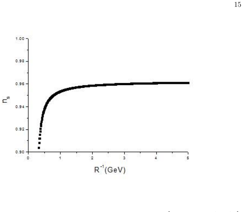
The central discovery is a direct link between the geometry of two moving branes and the temperature felt by an inflaton field. In the brane-antibrane system the apparent horizon sits at r_{\mathrm{horizon}} = cR/\dot R, where R is the orbital separation and \dot R its rate of change. Quantizing the inflaton in Kruskal coordinates and tracing over the inside of the horizon produces the thermal occupation number \langle B\rangle = $e^{{-2\pi r_{\mathrm{horizon}}$}\omega}/(1-$e^{{-2\pi r_{\mathrm{horizon}}$}\omega}), so the horizon radius acts as an inverse temperature. Substituting this distribution into the standard warm-inflation equations, the paper obtains H, \epsilon, \eta, the number of e-folds, and the scalar and tensor power spectra as functions of R and \dot R. The observed scalar amplitude from WMAP7, together with the standard point N\simeq 50 and n_s\simeq 0.96 located inside 0.01 < R_{\mathrm{tensor-scalar}} < 0.22, fixes the separation as R = (1.5\,\mathrm{GeV})^{-1} in intermediate inflation and R = (0.02225\,\mathrm{GeV})^{-1} in logamediate inflation.
Load-bearing premise
The load-bearing premise is that the apparent horizon of the accelerating brane pair is correctly identified as r_h = cR/\dot R and that the Kruskal-coordinate quantization used for a time-dependent brane separation remains valid; if that treatment fails, all predictions expressed through R lose their foundation.
Editorial extensions
If this is right
- Brane separation becomes an observable: if the central claim is correct, CMB measurements can constrain the distance between our brane and another brane in extra dimensions.
- Smaller separations strengthen inflation: as R shrinks, the interaction potential and horizon temperature rise, more inflatons are produced, and the number of e-folds grows in both intermediate and logamediate scenarios.
- The standard cosmological point picks out a specific length scale: N ≈ 50 with n_s ≈ 0.96 and 0.01 < R_T < 0.22 translates to R = (1.5 GeV)^{-1} (intermediate) or R = (0.02225 GeV)^{-1} (logamediate).
- Warm inflation needs no separate reheating epoch; the radiation bath is present throughout, so the brane-interaction signature appears directly in the perturbation spectra.
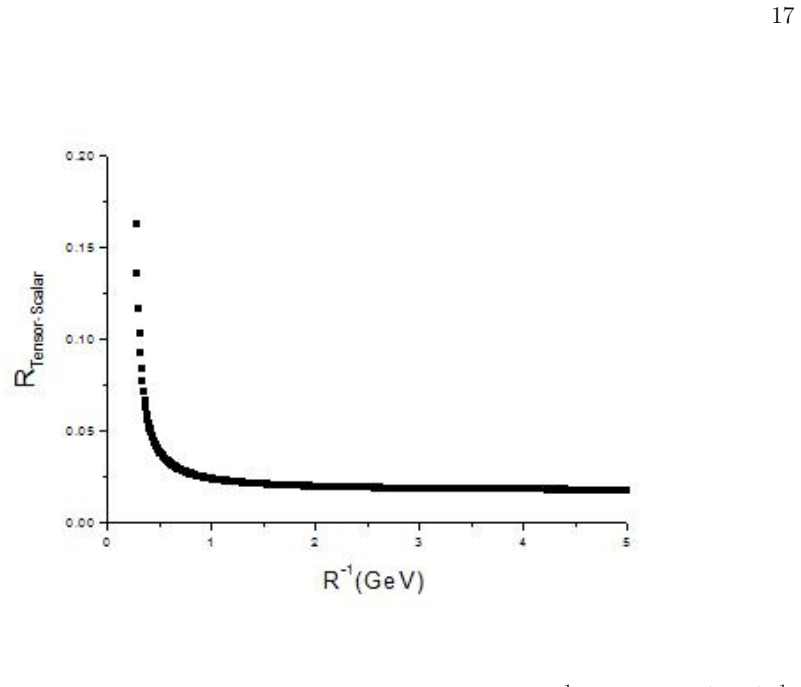
- The tensor-scalar ratio increases with R while the spectral index decreases, giving a monotonic relation that future CMB data can test.
Reading between the lines
- If the horizon-temperature identification survives, the two inflation models place the second brane at very different distances, by a factor of about 67; high-precision measurements of n_s and R_T could therefore discriminate between intermediate and logamediate inflation without any particle-physics assumption.
- The same construction should apply to more general multi-brane or non-parallel configurations; if so, warm inflation becomes a probe of the shape of the extra-dimensional potential, not just one separation.
- Because R and \dot R both enter, the model predicts a consistency relation between observables at different e-folds; checking whether the implied R trajectory is self-consistent across N would be a sharp test.
- The paper notes in the discussion that newer observational data should also fit; using more recent CMB measurements in place of WMAP7 would be a direct numerical extension of the paper's own formulas.
Signed reviews
Editorial analysis
A structured set of objections, weighed in public.
Referee Report
Summary. The paper proposes that the thermal distribution of inflatons in a brane-antibrane system, computed near the apparent horizon r_h = cR/\dot R, depends on the orbital separation R between the branes. It combines this distribution with the warm-inflation formalism to express the Hubble parameter, slow-roll parameters, spectral index, and tensor-scalar ratio in terms of R, and then uses the WMAP7 scalar amplitude to infer R = (1.5 GeV)^{-1} for intermediate inflation and R = (0.02225 GeV)^{-1} for logamediate inflation. The claimed result is that CMB data can therefore reveal the presence and separation of other branes.
Significance. The basic idea of linking extra-dimensional brane separation to warm-inflationary observables is attractive, and a valid derivation would give a concrete way to probe brane physics cosmologically. However, the central quantum-field-theory step contains an internal inconsistency, and the subsequent mapping from field quantities to brane-orbital quantities is asserted rather than derived. The quantitative claims therefore are not currently supported, although the conceptual direction could be interesting if the derivation were corrected and made verifiable.
major comments (4)
- [Section II, Eqs. (14) and (20)] There is an internal inconsistency in the derivation of the thermal distribution. Equation (14) defines tanh r = e^{-2π r_h ω}. From the normalized two-mode squeezed state in Eq. (19), the occupation number inside the horizon is ⟨α_in† α_in⟩ = sinh²r = tanh²r/(1−tanh²r) = e^{-4π r_h ω}/(1−e^{-4π r_h ω}). Equation (20) instead states ⟨B⟩ = e^{-2π r_h ω}/(1−e^{-2π r_h ω}). The factor of two in the exponent propagates through every subsequent expression that uses Eq. (20), including Eqs. (31)–(56), so the quoted numerical values R=(1.5 GeV)^{-1} and R=(0.02225 GeV)^{-1} are not solutions of the equations as written. In addition, Eq. (13) has tanh r = e^{-2 r_h ω} without the factor π, so the preceding equations are not mutually consistent either.
- [Section III, Eq. (23)] Equation (23) replaces the inflaton field B and its derivatives by expressions in R, \dot R, and \ddot R without any derivation. Starting from ⟨B⟩ = e^{-2π r_h ω}/(1−e^{-2π r_h ω}) with r_h = cR/\dot R, it is not shown how V(R,\dot R) = m²(1−\dot R/(2πω R))² or the terms involving \ddot R in the dynamical equations arise. This is a load-bearing step because all subsequent slow-roll, perturbation, and e-fold formulas in Section III are written in terms of R through this replacement; without the derivation, the connection between brane separation and CMB observables is not established.
- [Section III, Eq. (31)] The Hubble parameter in Eq. (31) is introduced after the statement 'From Eqs. (20), (24), (25), (26), (27) and (29) we obtain', but the derivation is not presented. In particular, the solution B(t)=B0 exp(\barω t^{(5f+2)/8}) appears in the same equation without explanation, and the slow-roll parameters and spectra in Eqs. (32)–(45) are built on this expression. The absence of the intermediate algebra prevents the reader from verifying the exponent (5f+2)/8, the normalization of \barω, and the resulting parameter chain.
- [Section III, after Eq. (41)] The inference of R is a fit, not a prediction, and its robustness is not demonstrated. Immediately after Eq. (41), the paper states that with A=1, f=1/2, \dot R=0.1, ω=4.6 GeV, and Γ0=1, Eq. (40) gives R=(1.5 GeV)^{-1}. No parameter scan, error propagation, or comparison with prior constraints on these constants is provided, and the abstract's language of a 'signature' is not supported. A meaningful claim would require showing how R varies over the allowed ranges of the free parameters; as it stands, the numerical value is a single point in a high-dimensional parameter space.
minor comments (4)
- [Throughout] There are numerous typographical errors and repeated words ('tthe', 'the the', 'inflaton'), and the notation oscillates between r_h, r_horizon, r0,horizon; a careful copyedit is needed.
- [Section II, Eq. (12)] Equation (12) contains an apparent typo: the region-II expression (\bar u/2r_h)^{-i2r_h r_h} should likely be (\bar u/2r_h)^{-i2r_h ω}.
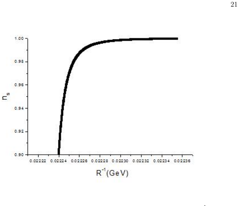
- [Figures 1–6] The figures would be more informative with axes labeled in physical units and with a brief description of how the curves depend on the chosen parameter values; as published, the reader cannot tell which curves correspond to the quoted R values.
- [References] Several references appear incomplete or not well matched to the citations in the text; please verify all citation-reference correspondences, especially for [3], [4], and the warm-inflation review entries.
Circularity Check
No significant circularity: the brane separation is fitted to the WMAP7 scalar-amplitude normalization, and the spectral-index and tensor-scalar comparisons are independent checks.
full rationale
The derivation chain is self-contained. The thermal distribution <B> in Eq. (20) is derived from the Kruskal-mode analysis of the brane-antibrane horizon (Eqs. (10)-(19)), with horizon radius r_h=cR/dotR from Eq. (9); the warm-inflation formulas are taken from the external literature [5,9,10]. The scalar amplitude Delta_R^2(R) in Eq. (40) is then equated to the WMAP7 normalization in Eq. (41), and the quoted brane separations R=(1.5 GeV)^{-1} and R=(0.02225 GeV)^{-1} are obtained by solving that equation after fixing the auxiliary constants. This is a parameter-estimation step, not a prediction: the R values are not used to predict the same amplitude that fixed them. The subsequent spectral index and tensor-scalar ratio are evaluated at the fitted R and compared with WMAP7 and Planck data, so they provide independent consistency checks. No load-bearing self-citation appears; refs [4,6,7] are external prior work, and the paper does not invoke a uniqueness theorem from its own author. A separate concern is that Eq. (20) appears inconsistent with the squeezed-state occupation number derived from Eq. (19), involving a factor of two in the exponent, but that is an internal mathematical error rather than a circular reduction: Eq. (20) is not equivalent to its inputs by construction, it contradicts them. Hence the circularity score is 0.
Assumptions & free parameters
free parameters (10)
- f =
1/2
- A =
1
- Gamma_0 =
1
- omega =
4.6 GeV
- R_0 =
0.45 GeV^-1
- dot_R_0 =
0.01
- dot_R =
0.1
- C =
70
- lambda =
10
- m
assumptions (5)
- domain assumption Unruh/Hawking quantization applies to the apparent horizon of the brane-antibrane system, yielding the thermal distribution of Eq (20).
- domain assumption The warm inflation equations of Bastero-Gil and Berera [5] hold when the inflaton field is represented by the thermal average <B>.
- domain assumption The apparent horizon radius is r_h = cR/\dot R.
- domain assumption The intermediate and logamediate scale factors a(t)=a_0 exp(A t^f) and a(t)=a_0 exp(A (ln t)^λ) describe the background expansion during inflation.
- domain assumption The brane-antibrane interaction potential is V(R) ~ 64π^2 μ^4 / 27 with μ^4 = 27/(32π^2) T_3 h^4 and h(R)=b^4/R^4.
Cite this review
Pith. "Pith review of Emergence of warm inflation in curved space-time between accelerating branes." pith.science (2026). https://pith.science/paper/JBVCJWJG
@misc{pith2026190809190,
  author       = {Pith},
  title        = {Pith review of: Emergence of warm inflation in curved space-time between accelerating branes},
  year         = {2026},
  howpublished = {\url{https://pith.science/paper/JBVCJWJG}},
  note         = {Machine review of arXiv:1908.09190}
}
read the original abstract
It appears that having our own brane to somehow interact with other branes could give rise to quite an interesting system and that that interaction could lead to some observable effects. We consider the question of whether or not these signatures of interaction between the branes can be observed. To answer this question, we investigate the effect induced by the inflaton in the WMAP7 data using the warm inflationary model. In this model, slow-roll and perturbation parameters are given in terms of the inflaton thermal distribution. We show that this distribution depends on the orbital radius of the brane motion under the interaction potential of other branes in extra dimensions. Thus, an enhancement in the brane inflation can be a signature of an orbital motion in extra dimensions and consequently, some signals of other branes can be detected by observational data. According to experimental data, the N = 50 case leads to ns = 0:96, where N and ns are the number of e-folds and the spectral index, respectively. This standard case may be found in the range 0:01 < R(Tensor-scalar) < 0:22, where R(Tensor-scalar) is the tensor-scalar ratio. We find that at this point, the radial distance between our brane and another brane is R = 1/(1:5GeV ) in intermediate, and R = 1/(0:02225GeV ) in logamediate inflation.
Figures

Figures from the paper (3 more)


Reference graph
Works this paper leans on
-
[1]
(30) where t1 is the begining time of inflation. From Eqs.(20), (24), (25), (26), (27) and (29) we obtain the Hubble parameter as: H =fA(ln<B >− ln<B 0 > ¯ω ) 8(f−1) 5f +2 = fA( ln e−2πrhorizonω 1−e−2πrhorizonω− ln e−2πr0,horizonω 1−e−2πr0,horizonω ¯ω ) 8(f−1) 5f +2 ∼ fA( −2πω(rhorizon−r0,horizon) + ln 1−e−2πr0,horizonω 1−e−2πrhorizonω ¯ω ) 8(f−1) 5f +2 ∼ ...
-
[2]
It is clear that the number of e-folds N is much larger for a smaller orbital radial distance between the branes. This is because, as the distance between the branes becomes smaller, the temperature becomes larger and the thermal radiation of the inflatons enhances. Now, we will consider tensor and scalar perturbations that appear during the inflationary pe...
-
[3]
Alireza Sepehri, Somayyeh Shoorvazi, Mohammad Ebrahim Zomorrodian, Can. J. Phys., 91: 256-259, (2013)/ Can. J. Phys. 87, 1151-1158 (2009)
work page 2013
-
[4]
As can be seen from Fig.2, the spectral index decreases rapidly when the distance between the branes increases. By comparing Fig. 1 and Fig. 2, we find that the N≃ 50 case leads to ns≃ 0.96. This result is compatible with observational data [5, 20, 22]. At this point, the radial distance between our brane and another brane is R = (1.5GeV )−1. Using Eq.(20)...
-
[5]
We observe that as the orbital radius distance between branes increases, the tensor-scalar ratio increases. By comparing Figs. 2 and 3, we notice that the standard case ns≃ 0.96, may be found in 0.01 < RTensor−scalar < 0.22, which agrees with observational data [5, 20, 22]. At this stage, the radial distance between our brane and another brane is R = (1.5...
-
[6]
In this case, like the intermediate case, we find that the number of e-folds N and the spectral index are much larger for smaller orbital radial distance between branes. This is because, as the distance between the branes becomes smaller, the temperature becomes larger, and the thermal radiation of the inflatons enhances. Finally, we could find the tensor-sc...
-
[7]
In this case, like the intermediate case, with an increase in the orbital radial distance between branes, the tensor-scalar ratio increases. By comparing Figs. 5 and 6, we notice that the standard case ns≃ 0.96, may be found in 0.01<R tensor−scalar < 0.22, which agrees with observational data [5, 20, 22]. At this stage, the radial distance between our bra...
-
[8]
Salvador Robles-Perez, Pedro F. Gonzalez-Diaz, Phys. Rev. D81: 083529, (2010)
work page 2010
Show all 32 references
-
[9]
Gonzlez-Diaz, Salvador Robles-Perez, Phys
Pedro F. Gonzlez-Diaz, Salvador Robles-Perez, Phys. Lett. B679: 298-301, (2009)
2009
-
[10]
Bastero-Gil, A
M. Bastero-Gil, A. Berera, R. O. Ramos and J. G. Rosa, JCAP 1301, 016 (2013)
2013
-
[11]
Yin-Zhe Ma, Qing-Guo Huang, Xin Zhang, , Phys. Rev. D., 87, 103516, (2013)
2013
-
[12]
Mar Bastero-Gil, Arjun Berera, Int. J. Mod. Phys. A 24: 2207-2240, (2009)
2009
-
[13]
N. D. Birrell and P. C. W. Davies, Quantum fields in curved space (Cambridge University 23 Press, New York, 1982)
1982
-
[14]
Doyeol Ahn, Phys. Rev. D74: 084010, (2006)
2006
-
[15]
Sepehri, S
A. Sepehri, S. Shoorvazi, Astrophysics and Space Science, 344, 521-527, (2013)
2013
-
[16]
Bastero-Gil, A
M. Bastero-Gil, A. Berera and R. O. Ramos, JCAP 1109, 033 (2011)
2011
-
[17]
J. D. Barrow, A. R. Liddle, Phys. Rev. D47, 5219, (1993)
1993
-
[18]
Berera, Phys
A. Berera, Phys. Rev. Lett. 75, 3218 (1995) [astro-ph/9509049]; Phys. Rev. D55, 3346 (1997) [hep-ph/9612239]
1995 arXiv
-
[19]
J. D. Barrow, Class. Quantum Grav. 13, 2965 (1996)
1996
-
[20]
This result is consistent with previous calculations [21]
as: ∆2 R = (2.455± 0.096)× 10−19 (41) Using this equation and equation(40), and choosing (A=1, f=1/2, ˙R = 0.1, ω = 4.6(GeV ), Γ0=1), we obtain the radial distance between our brane and another brane,R = (1.5GeV )−1. This result is consistent with previous calculations [21]. A...
-
[21]
J. D. Barrow, Phys. Rev. D 51, 2729 (1995)
1995
-
[22]
Mar Bastero-Gil Arjun Berera, Phys. Rev. D76: 043515, 2007
2007
-
[23]
Yokoyama and K
J. Yokoyama and K. Maeda, Phys. Lett. B207, 31, (1988)
1988
-
[24]
J. D. Barrow, Phys. Lett. B235, 40 (1990); J. D. Barrow and P. Saich, Phys. Lett. B249, 406 (1990)
1990
-
[25]
A. H. Guth and S. Y. Pi, Phys. Rev. Lett. 49, 1110 (1982)
1982
-
[26]
V. F. Mukhanov and G. V. Chibisov, Pisma Zh. Eksp. Teor. Fiz. 33, 549 (1981) [JETP Lett. 33, 532 (1981)]; S. W. Hawking, Phys. Lett. B 115, 295 (1982); A. A. Starobinsky, Phys. Lett. B 117, 175 (1982); J. M. Bardeen, P. J. Steinhardt and M. S. Turner, Phys. Rev. D 28, 679 (1983)
1981
-
[27]
Komatsu et al
E. Komatsu et al. arXiv:1001.4538 [astro-ph.CO]; B. Gold et al., arXiv: 1001.4555 [astro- ph.GA]; D. Larson et al., arXiv: 1001.4635 [astro-ph.CO]
-
[28]
Belanger, A
G. Belanger, A. Belyaev, M. Brown, M. Kakizaki and A. Pukhov, Phys. Rev. D87, 016008 (2013)
2013
-
[29]
Ade et al
P. Ade et al. (Planck Collaboration), Astron. Astrophys. 536, 16464 (2011); P. Ade et al. astro-ph/0604069; URL http://www.rssd.esa.int/index.php?project=Planck
2011 arXiv
-
[30]
P. J. E. Peebles and B. Ratra, Rev. Mod. Phys. 75, 559 (2003)
2003
-
[31]
P. G. Ferreira and M. Joyce, Phys. Rev. D 58, 023503 (1998)
1998
-
[32]
Eds. M. Abramowitz and I. A. Stegun, Handbook of Mathematical Functions with Formulas, Graphs, and Mathematical Tables (Dover, 1972), 9th printing; G. Arfken, The incomplete gamma function and related functions, Mathematical Methods for Physicists, 3rd edn. (Aca- demic Press, 1985)
1972
Reviewed August 14, 2026 · model on record in the stance chip above.
Discussion (0). Continue with ORCID to comment.