Effects of random fields on the reversal of magnetisation of Ising ferromagnet

Moumita Naskar; Muktish Acharyya

REVIEW 3 major objections 5 minor 37 references

Effects of random fields on the reversal of magnetisation of Ising ferromagnet

T0 review · 3 major / 5 minor · reviewed 2026-08-14 · deepseek-v4-flash

Challenge this review Re-run · record.json Download PDF Read on arXiv ↗ Review JSON

Pith's one-line read Adding quenched random fields to a uniform field reduces the magnetisation reversal time in the 2D Ising ferromagnet, and bimodal disorder does so most effectively.

desk verdict The main observation—quenched random fields shorten magnetization reversal time in 2D Ising—is solid and supported by multiple figures, but the cross-distribution comparison is undercut by an inconsistent Gaussian width convention. read the letter →

arxiv 1908.09268 v4 pith:5S3AMSOV submitted 2019-08-25 cond-mat.stat-mech

Moumita Naskar , Muktish Acharyya This is my paper · ORCID

classification cond-mat.stat-mech MSC 82C2082C4482C80 PACS 75.60.Jk75.10.Hk05.10.Ln

keywords IsingferromagnetMonteCarlosimulationMetropolissinglespinflipalgorithmQuencheddisorderClassicalnucleationtheorymagnetisationreversalAvramilawbimodaldistribution

verification ladder T0 review T1 audit T2 compute T3 formal

The pith

A machine-rendered reading of the paper's core claim, the machinery that carries it, and where it could break.

The reading

This paper uses Monte Carlo simulations of a two-dimensional Ising ferromagnet to ask whether a quenched random magnetic field, added to a uniform reversing field, changes how long the magnetisation takes to flip. It reports that any zero-mean random-field distribution (bimodal, uniform, or Gaussian) shortens the reversal time compared with the uniform field alone, with the bimodal distribution the most effective. The reversal time falls exponentially with the width of the random-field distribution, while the metastable volume fraction still follows Avrami's $t^3$ law. For large disorder widths the single-droplet nucleation regime disappears and reversal proceeds by growth and coalescence of many droplets. The motivation is that faster, controllable switching matters for magnetic storage and recording.

What carries the argument

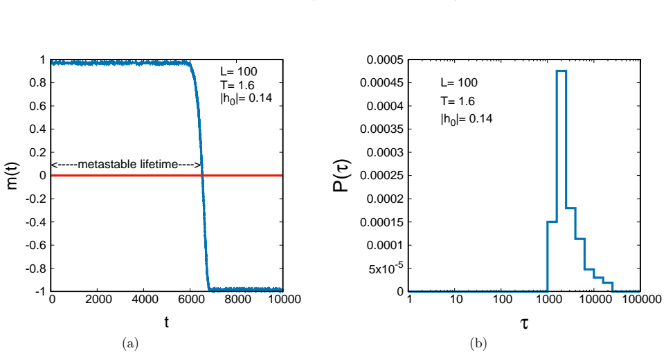
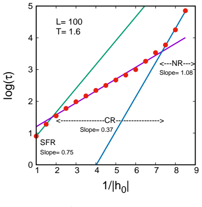
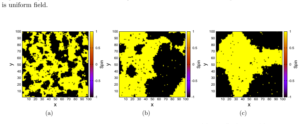
The central object is the two-dimensional Ising ferromagnet with Hamiltonian $H = -J \sum_{\langle i,j\rangle} S_i S_j - \sum_i h_i S_i$, where $h_i = h_0 + h_r$ is a uniform field plus a quenched random field drawn from one of three zero-mean distributions (bimodal, uniform, or Gaussian). Dynamics is Metropolis single-spin-flip Monte Carlo, and the reversal time $\tau$ is defined as the first time the magnetisation becomes negative starting from a fully ordered state. The argument is carried by the Becker-Doring classical nucleation relation $\log \tau \sim 1/|h|^{d-1}$ in the single-droplet regime and $\sim 1/((d+1)|h|^{d-1})$ in the coalescence regime, together with the Avrami law for the metastable volume fraction. These supply the diagnostics: slopes in the $\log \tau$ versus $1/|h|$ plot identify the strong-field, coalescence, and nucleation regimes, and spin snapshots at reversal distinguish single-droplet from multidroplet growth.

What would settle it

Re-run the reversal-time comparison with all three distributions normalised to the same standard deviation (for example, set the Gaussian $\sigma$ equal to the standard deviation of the uniform and bimodal distributions at each $w$), and measure $\log \tau$ versus $1/|h_0|$ at $L=100$, $T=1.6$, $|h_0|=0.125$ for $w$ from $0.45$ to $0.5$; if the single-droplet regime still survives for uniform and Gaussian disorder at $w=0.5$, or if the Gaussian ranking reverses once its width is matched, the reported thresholds and ranking would not hold.

Watch

Extended reading notes

Core claim

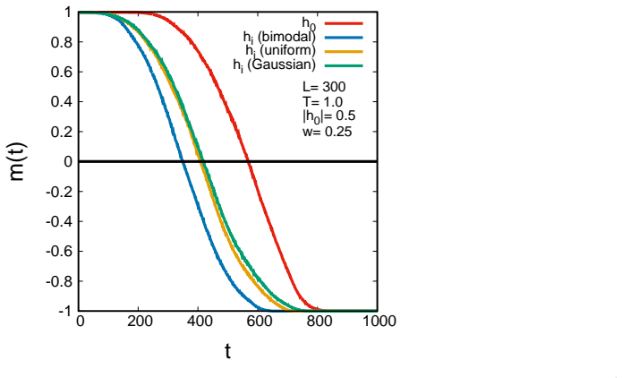
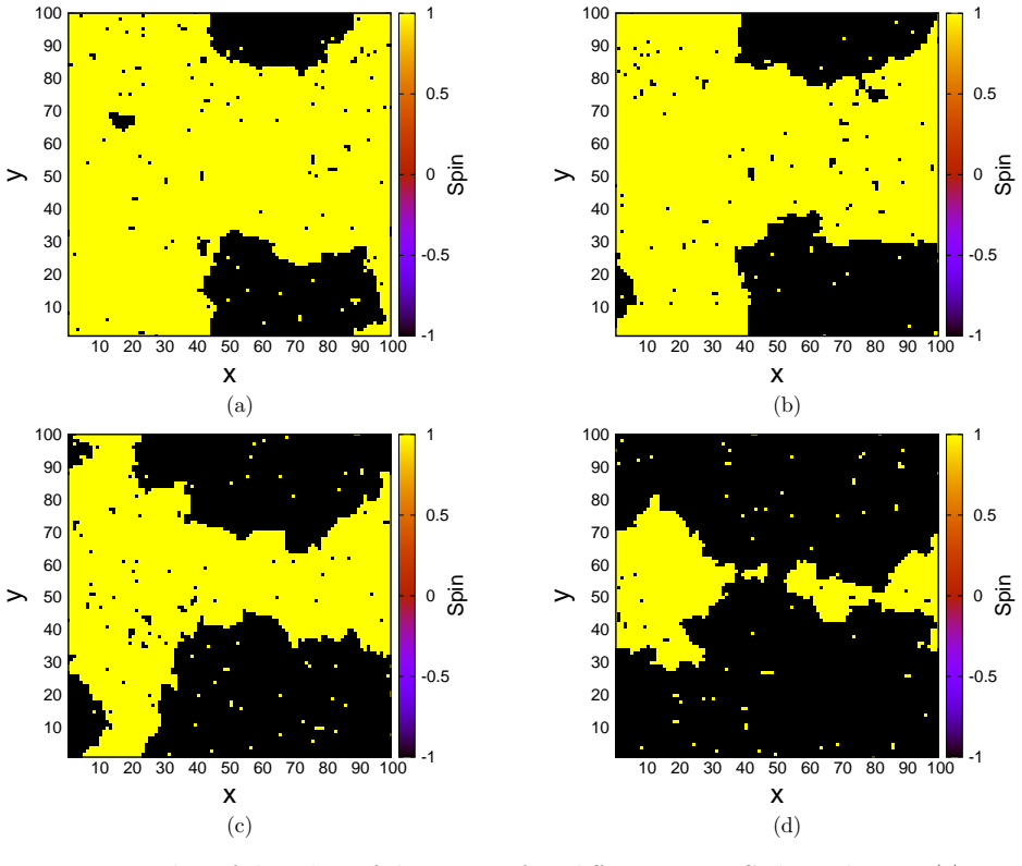
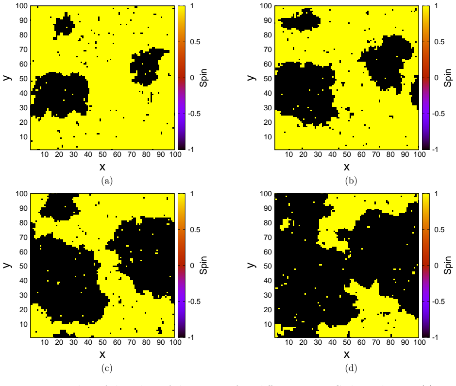
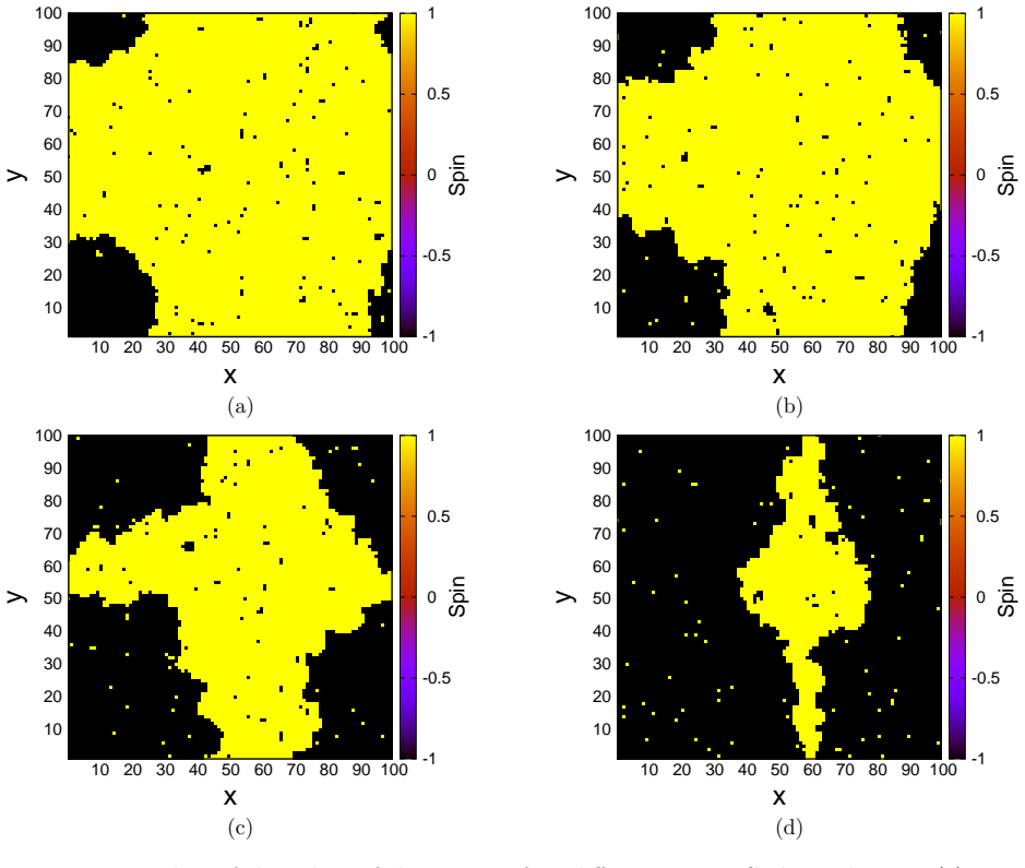
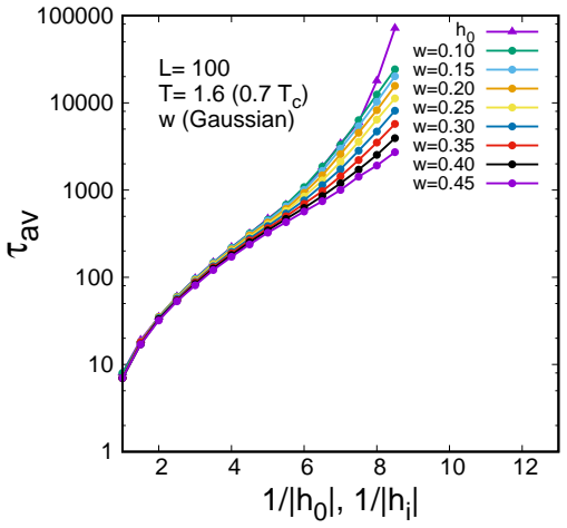
In the two-dimensional Ising ferromagnet below the Curie temperature, adding a site-dependent but time-independent random field of zero mean to the applied uniform field systematically reduces the reversal time for all three distributions studied, and the reduction is largest for the bimodal distribution. Mean and most-probable reversal times both follow $\exp(-B w)$ in the disorder width $w$ and $\exp(A/T)$ in inverse temperature. The decay of the metastable volume fraction obeys the Avrami $t^3$ law, just as in the pure case. Becker-Doring analysis shows that the strong-field and coalescence regimes survive the addition of random fields, but the single-droplet nucleation regime is progressively destroyed as $w$ grows; for bimodal disorder it disappears between $w=0.3$ and $w=0.35$ at $|h_0|=0.125$ and $T=1.6$, while for uniform and Gaussian disorder it survives up to at least $w=0.45$.

Load-bearing premise

The comparison across disorder types assumes that $w$ means the same thing for all three distributions, but the Gaussian is described in the text as having standard deviation $\sigma=2w$ while the Fig. 5 caption says $\sigma=w/5$; if the text value is correct, the Gaussian disorder at a given $w$ is much broader than the bimodal and uniform disorder, so the effectiveness ranking and the reported loss of the nucleation regime are not controlled comparisons.

Editorial extensions

If this is right

Adding quenched disorder of any of the three zero-mean forms shortens the reversal time, so disorder width can serve as a control knob for switching speed rather than only a source of noise.
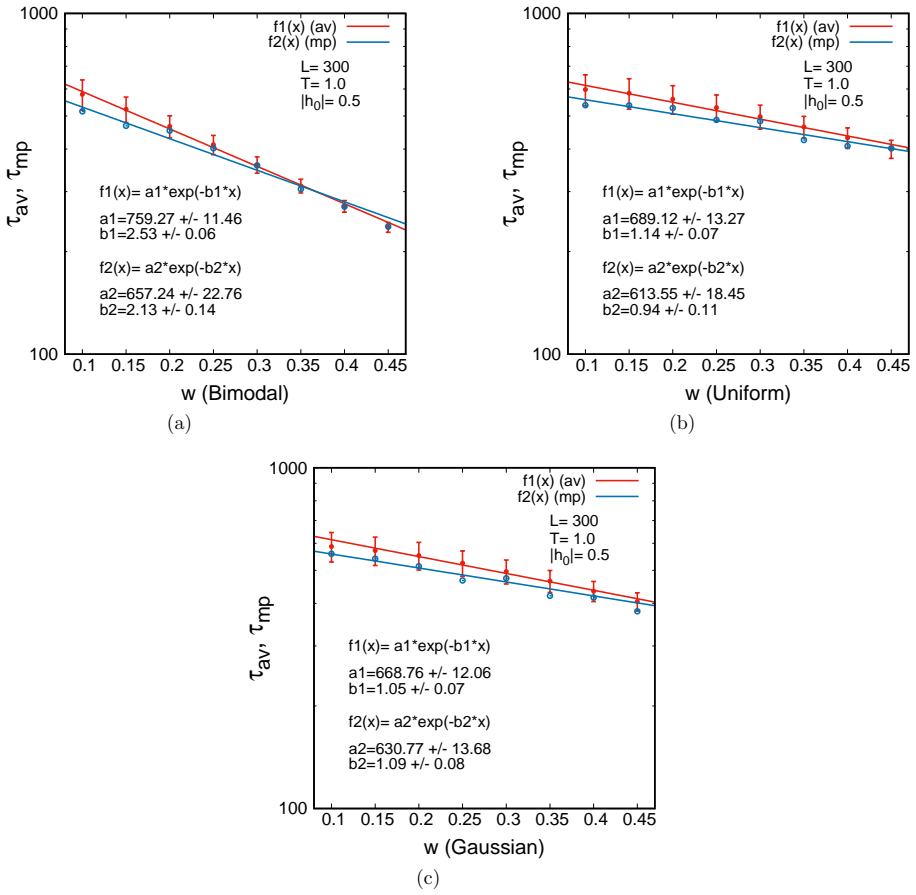
The exponential dependence $\tau \sim \exp(-B w)$ means modest increases in disorder width produce large reductions in reversal time; the fitted decay constants are roughly twice as large for bimodal disorder as for uniform or Gaussian disorder at $T=1.0$ and $|h_0|=0.5$.
Bimodal disorder is the most effective of the three distributions studied, and the snapshots show it changes reversal morphology from single-droplet to multidroplet growth already by $w=0.35$ at $|h_0|=0.125$.
For sufficiently large random-field width the single-droplet nucleation regime disappears, so the Becker-Doring single-droplet scaling no longer describes reversal; the coalescence description still applies.
At higher temperatures the reversal-time distributions for the three disorder types converge, indicating that thermal fluctuations dominate over the details of the random-field distribution.

Reading between the lines

Editorial extensions of the paper, not claims the author makes directly.

A controlled comparison that matches the standard deviations of all three distributions would likely change the reported ranking and the critical width for loss of the nucleation regime; the manuscript is internally inconsistent about the Gaussian width (text says $\sigma=2w$, Fig. 5 caption says $\sigma=w/5$).
If the equivalence between disorder width and temperature is taken seriously, engineered binary disorder could lower switching times without raising temperature, a design route for magnetic storage that the paper only gestures at.
The disappearance of the single-droplet regime for bimodal disorder suggests a testable scaling: the critical width beyond which nucleation disappears should scale with $|h_0|$, since the mechanism is local fields opposing droplet growth; the paper does not derive this scaling.
The finite-size check of the exponential $\tau(w)$ decay is performed only for bimodal disorder; repeating it for uniform and Gaussian disorder at $L=400$ would show whether the reported thresholds are size-dependent.

Share X Bluesky LinkedIn Reddit HN

Signed reviews

No signed human review yet.

Editorial analysis

A structured set of objections, weighed in public.

Desk editor's note, referee report, and a circularity audit.

Desk Editor's Note

read the letter

The headline is true: adding quenched random fields to the uniform-field Ising model does shorten the reversal time, and this is shown consistently across several independent figures (Figs. 7, 9, 13, 16, 18). That part of the paper I trust. What is new is the systematic comparison of three zero-mean disorder distributions (bimodal, uniform, Gaussian) for reversal dynamics, which I haven't seen in the cited literature. The authors also check Avrami behavior and the Becker-Doring slope structure, and they include a finite-size check for the bimodal case. Those are all legitimate and give the paper real content.

The soft spots are real but localized. The worst is the Gaussian width definition. Section III says sigma = 2w is used throughout, while the Fig. 5 caption says the plotted Gaussian has sigma = w/5 and only parenthetically notes that "in our work we have used sigma = 2w." At fixed w, these differ by a factor of 10 in sigma. That matters directly for the ranking claim that bimodal is the most effective disorder: if sigma = 2w, the Gaussian is far broader than bimodal or uniform at the same nominal w, so the comparison is not controlled. If sigma = w/5, the Gaussian is almost negligible disorder, which explains why the nucleation regime persists at w = 0.45 but makes that persistence uninformative. Either way, the cross-distribution ranking and the threshold for losing the nucleation regime are not established on a common disorder scale. The qualitative decrease of reversal time is not endangered, but the quantitative comparison is.

Other issues are minor by comparison. The fitted slopes in the SFR/CR/NR regimes and the Avrami reference lines lack error bars; the regime boundaries are visually placed. No code or data are provided, so reproducibility is limited. The exponential fits for tau(T) and tau(w) are descriptive, not presented as predictions, so that's fine. The Becker-Doring analysis is checked against external slope relations, not self-derived, so circularity is not a concern.

Who should read this: people working on magnetization reversal in kinetic Ising models or on disorder effects in metastable decay. It is not a breakthrough, but it is a legitimate parameter scan with a clear physical question. A serious referee should see it, and with a request to fix the Gaussian convention and provide error bars or at least state the actual sigma used in each figure, it could be acceptable. I would not cite it in my own next-year work, but I would probably bring it to a reading group for the discussion of how disorder strength should be defined.

Recommendation: send it to peer review, not desk reject. The main observation is likely correct and the paper is honest enough to be worth engaging with despite the internal inconsistency.

Referee Report

3 major / 5 minor

Summary. This manuscript reports Monte Carlo simulations of magnetization reversal in a two-dimensional Ising ferromagnet driven by a uniform field plus quenched random fields drawn from bimodal, uniform, and Gaussian distributions. The central observations are that any zero-mean random field reduces the reversal time relative to the uniform-field-only case, that the bimodal distribution appears most effective among the three considered, that reversal times decay roughly exponentially with temperature and with disorder width, that the metastable volume fraction follows an Avrami-type law, and that for sufficiently large disorder width the single-droplet nucleation regime disappears at weak uniform field. The paper compares the measured slopes of log-reversal-time versus inverse field with Becker-Doring predictions for the strong-field, coalescence, and nucleation regimes.

Significance. If the quantitative claims are established, the paper would be a useful contribution to the study of metastable decay in disordered Ising systems: the qualitative effect of quenched random fields in shortening reversal time is robust and is supported by several independent figures (Figs. 7, 9, 13, 16, and 18), and the finite-size check in Fig. 12 is a commendable feature. The explicit fits in Figs. 10 and 11 provide concrete parameterizations of the temperature and width dependence. However, the cross-distribution comparisons are not currently controlled because the Gaussian width is defined inconsistently, and the regime classification and slope estimates lack objective criteria and error bars. These issues directly affect the quantitative ranking of the disorder distributions and the reported threshold for loss of the nucleation regime, so the manuscript needs major revision before the quantitative claims can be accepted.

major comments (3)

[Section III, Eq. (12c) and Fig. 5 caption] The definition of the Gaussian disorder width is inconsistent. The text after Eq. (12c) states that sigma = 2w is 'considered throughout our work', while the Fig. 5 caption describes the plotted Gaussian random field as having sigma = w/5 and adds parenthetically that sigma = 2w was used in the work. The sentence following Eq. (12c) also says that the random-field values are distributed between -w and w, which is not true for an unbounded Gaussian. Because Figs. 7, 11, and 13-19 use w as the common control parameter, the comparison of bimodal, uniform, and Gaussian disorder is not controlled: at w = 0.45, the Gaussian standard deviation is either 0.9 or 0.09, leading to opposite interpretations of why the nucleation regime persists in Fig. 18. Please specify the exact sigma used in every simulation, and either replot the cross-distribution comparisons using a common measure of disorder strength (such as the standard deviation or a common interquartile range) or explicitly restrict the Gaussian ranking claims to the chosen convention.
[Section IV, Figs. 13, 15, 16, and 18] The claim that the nucleation regime disappears for bimodal disorder between w = 0.30 and w = 0.35 but persists for uniform and Gaussian disorder at w = 0.45 is a central quantitative result, yet it is supported only by visual inspection of the log tau versus 1/|h| curves and by a small number of snapshots. No criterion is given for classifying a curve as possessing a nucleation regime, and the slopes in the purported SFR, CR, and NR regions are not fitted with error bars for the disordered cases. Please define an objective classifier (for example, a slope ratio close to 1/3 between the CR and NR regions, a curvature threshold, or a droplet-count measurement) and report the uncertainties in the fitted slopes and in the inferred critical width.
[Section IV, Figs. 3, 13, 16, and 18] The comparison with Becker-Doring theory rests on the fitted slopes in the three regimes, but the pure-system slopes are quoted without uncertainties (Fig. 3: 0.75, 0.37, 1.08) and the disordered-system curves in Figs. 13, 16, and 18 are not fitted at all. Consequently, the statement that the coalescence-regime slope is approximately one third of the nucleation-regime slope, and the assertion that this relation survives in the presence of random fields, cannot be quantitatively assessed from the presented data. Please provide least-squares fits with confidence intervals for each regime and state how the regime boundaries were chosen.

minor comments (5)

[Section III, after Eq. (12c)] The phrase 'distributed between -w to w' is inaccurate for the Gaussian distribution; please rephrase to describe the standard deviation or a quantile range.
[Fig. 4 caption] The caption writes '1/h0 = -1.5' and similarly for the other regimes, but the axis labels use positive 1/|h0|; the signs are inconsistent and should be corrected to 1/|h0| = 1.5, 4.5, and 8.0.
[Fig. 12 and Section IV] The decay exponent for L = 100 (b = 4.21) differs strongly from the values for L = 200-400 (b between 2.42 and 2.62), so the statement that L = 300 is 'free from any finite size effect' is stronger than the data support; please discuss the L = 100 deviation or restrict the claim to larger system sizes.
[Section IV, near Fig. 6] There are typographical errors in the text, for example 'Acase for randomly distributed field thefter applying negative field'; the manuscript should be proofread for such issues.
[Section IV, Fig. 8 and surrounding text] The Avrami-law statement refers to the 'third power of time' and the figure label is (t/tau)^3; the text should consistently write t^3 and specify the functional form ln(N1/N) proportional to -(t/tau)^3.

Circularity Check

0 steps flagged · score 0.0 of 10

No circularity: reversal-time claims are direct Monte Carlo measurements checked against independent Becker-Doring and Avrami benchmarks; the Gaussian width inconsistency is a non-circular control concern.

full rationale

The paper's central quantitative results are not derived from fitted inputs. Reversal times are measured directly from Monte Carlo metastable decays (Fig. 2), and the Becker-Doring check (Fig. 3 and Eqs. 7-9) compares measured slopes (about 0.37 versus the predicted 1/3, and 1.08 in the nucleation regime) against an independent classical nucleation formula. The temperature and width dependences in Figs. 10-11 are descriptive exponential fits to simulation data, not predictions generated from those fits, so no fitted parameter is renamed as a predicted result. The Avrami-law check in Fig. 8 is an external benchmark, not an input to the simulation. The only self-citation, Ref. [5] in the coalescence-regime discussion, merely cross-references a prior paper for a formula that is re-derived in Eqs. (8)-(9) within the present paper; it is not load-bearing. There is a genuine internal inconsistency in the Gaussian-width convention: Eq. (12c) states sigma = 2w, while the Fig. 5 caption states sigma = w/5. That ambiguity undermines the controlled comparison across distributions and the location of the nucleation-regime crossover, but it is a correctness or reproducibility concern rather than a circular derivation: no claimed prediction is defined in terms of the data it purports to explain, and no input quantity is equivalent by construction to the output claim. Accordingly, no specific circular step can be exhibited, and the appropriate circularity score is 0.

Assumptions & free parameters 5 free parameters · 5 assumptions · 0 invented entities

No new physical entities are introduced. The central simulation relies on standard models and theories. The main ad hoc choices are the Gaussian width convention and the interpretation of linearity in inverse field as Becker-Doring validity; both affect the comparison across disorder distributions.

free parameters (5)

Arrhenius prefactor A and exponent B in tau ~ A exp(B/T) = A ~ 0.4-0.7, B ~ 6.3-7.1 per distribution (Fig. 10)
Two-parameter fits to mean and most-probable reversal times versus 1/T; no theoretical derivation of A and B.
Prefactor C and exponent D in tau ~ C exp(-D w) = C ~ 600-760, D ~ 0.94-2.53 per distribution (Fig. 11)
Empirical exponential fits to reversal time versus random-field width; central to the tunability claim.
Slopes of log tau versus 1/|h0| in SFR, CR, and NR = 0.75, 0.37, 1.08 (Fig. 3)
Used to identify regimes and support the Becker-Doring slope ratio; no error bars are reported.
Linear reference slope and intercept for Avrami plots = -0.712, -0.1 and -0.524, -0.202 (Fig. 8)
Reference lines drawn to support the Avrami t^3 law; not fits with reported uncertainty.
Gaussian standard deviation sigma relative to w = sigma=2w in text, sigma=w/5 in Fig. 5 caption
Hand-set relation; inconsistent between text and figure, and affects the cross-distribution comparison.

assumptions (5)

domain assumption The 2D Ising Hamiltonian with nearest-neighbor coupling J and local fields h_i = h0 + h_r describes the ferromagnet, and Metropolis dynamics samples the equilibrium distribution.
Standard model and algorithm; not derived in the paper.
domain assumption Becker-Doring classical nucleation theory: droplet free energy E_l = -2hl + sigma l^((d-1)/d), critical droplet size, nucleation rate I proportional to exp(-E_c/(kBT)), and reversal-time relations (7a) and (9a).
Imported from the cited literature and used as the benchmark to classify reversal regimes.
domain assumption Avrami law: metastable volume fraction decays as exp(-const * t^(d+1)).
Imported from the cited literature and used to analyze the decay curves.
ad hoc to paper For weak random fields, log tau versus 1/h0 remains linear with the theoretical slopes, and linearity is interpreted as validity of Becker-Doring theory in the disordered system.
The theory is derived for uniform fields; applying it with h0 only is an assumption tested visually rather than quantitatively.
ad hoc to paper The width parameter w is a common measure across the three distributions.
The Gaussian sigma=2w convention makes the nominal widths non-comparable; this assumption underlies the ranking of distributions.

how reviews work

0 comments

Cite this review

Pith. "Pith review of Effects of random fields on the reversal of magnetisation of Ising ferromagnet." pith.science (2026). https://pith.science/paper/5S3AMSOV

@misc{pith2026190809268,
  author       = {Pith},
  title        = {Pith review of: Effects of random fields on the reversal of magnetisation of Ising ferromagnet},
  year         = {2026},
  howpublished = {\url{https://pith.science/paper/5S3AMSOV}},
  note         = {Machine review of arXiv:1908.09268}
}

read the original abstract

We have studied the reversal time of the magnetisation in two dimensional Ising ferromagnet in the presence of externally applied uniform magnetic field using Monte Carlo simulation based on Metropolis single spin flip algorithm. Then we have investigated the change in reversal time due to the presence of quenched random field in addition to the uniform magnetic field. We report the results of statistical distribution of reversal times in the presence of three different types of the distributions (namely, uniform, bimodal and normal) of random fields and compared the results with those obtained for uniform field only. We have observed that the reversal time decreases due to the presence of any kind (of distribution) of the random fields. The metastable volume fraction is observed to follow the Avrami's law. Dependence of reversal times on temperature and different widths of the distributions of random fields are also reported. We have also checked whether the system obeyed Becker-Doring theory of classical nucleation in presence of additional random field and tried to investigate the range of the width of the distribution of random field. For larger width of the distribution of random field, the system fails to show the reversal via the nucleation of a single droplet (for small values of uniform field only). The possible reason is analysed.

Figures

Figures reproduced from arXiv: 1908.09268 by the authors.

**Figure 2.** (a) A typical decay of metastable state for lattice [PITH_FULL_IMAGE:figures/full_fig_p013_2.png] view at source ↗

**Figure 3.** log of mean reversal time with 1/h0 for lattice size L = 100 at temperature T = 1.6, where h is uniform field. 10 20 30 40 50 60 70 80 90 100 10 20 30 40 50 60 70 80 90 100 y x ’mn1_snap.dat’ -1 -0.5 0 0.5 1 Spin (a) 10 20 30 40 50 60 70 80 90 100 10 20 30 40 50 60 70 80 90 100 y x ’mn4_snap.dat’ -1 -0.5 0 0.5 1 Spin (b) 10 20 30 40 50 60 70 80 90 100 10 20 30 40 50 60 70 80 90 100 y x ’mn3_snap.dat’ -1 -0.5 0 0.5 1… view at source ↗

Figures from the paper (16 more)

**Figure 4.** Figure 4: Snapshots at the time of reversal in three regimes o [PITH_FULL_IMAGE:figures/full_fig_p014_4.png]

**Figure 5.** Figure 5: Image plots (zoomed in from L = 300 to L = 50) of the three different distributions of random field each of mean 0 and width w = 0.25, (a)Bimodal random field, (b)Uniformly distributed random field, (c)Gaussian random field with σ = w/5. 50 100 150 200 250 300 50 100 1…

**Figure 6.** Figure 6: Image plots of the values of the spins at the time of m [PITH_FULL_IMAGE:figures/full_fig_p015_6.png]

**Figure 7.** Figure 7: Variation of magnetisation with time at temperatu [PITH_FULL_IMAGE:figures/full_fig_p016_7.png]

**Figure 8.** Figure 8: logarithmic metastable volume fraction ( [PITH_FULL_IMAGE:figures/full_fig_p016_8.png]

**Figure 9.** Figure 9: Normalised distribution of reversal times for 100 [PITH_FULL_IMAGE:figures/full_fig_p017_9.png]

**Figure 10.** Figure 10: Variation of mean reversal time (τav) and most probable reversal time (τmp) with the inverse of temperature in presence of the random field hi ((a) bimodal (b) uniform and (c) Gaussian distribution). In each case, uniform field is h0 = −0.5 and the width of the random…

**Figure 11.** Figure 11: Variation of mean reversal time (τav) and most probable reversal time (τmp) with the width of random field hi (for (a) bimodal (b) uniform and (c) Gaussian distribution). In each case, uniform field is h0 = −0.5 and the temperature is T = 1.0, lattice size is L = 300.…

**Figure 12.** Figure 12: Variation of mean reversal time (τav) with the width of the random field hi (bimodal distribution) with different size of the lattice (L = 100, 200, 300, 400). In each case, uniform field is h0 = −0.5. 1 10 100 1000 10000 100000 2 4 6 8 10 12 L= 100 T= 1.6 (0.7 Tc ) …

**Figure 13.** Figure 13: Variation of the mean reversal time (in logarithm [PITH_FULL_IMAGE:figures/full_fig_p020_13.png]

**Figure 14.** Figure 14: Image plots of the values of the spins at four differe [PITH_FULL_IMAGE:figures/full_fig_p021_14.png]

**Figure 15.** Figure 15: Image plots of the values of the spins at four differe [PITH_FULL_IMAGE:figures/full_fig_p022_15.png]

**Figure 16.** Figure 16: Variation of mean reversal time (in logarithmic s [PITH_FULL_IMAGE:figures/full_fig_p023_16.png]

**Figure 17.** Figure 17: Image plots of the values of the spins at four differe [PITH_FULL_IMAGE:figures/full_fig_p024_17.png]

**Figure 18.** Figure 18: Variation of mean reversal time (in logarithmic s [PITH_FULL_IMAGE:figures/full_fig_p025_18.png]

**Figure 19.** Figure 19: Image plots of the values of the spins at four differe [PITH_FULL_IMAGE:figures/full_fig_p026_19.png]

Discussion (0). Continue with ORCID to comment.

Reference graph

Works this paper leans on

37 extracted references · 37 canonical work pages

[1]

Vogel, J

J. Vogel, J. Moritz, O. Fruchart, Comptes Rendus Physiqu e 7, 977-987 (2006)

work page 2006
[2]

S. N. Piramanayagam and T. C. Chong, Development in Data S torage: Material Perspective, Wiley- IEEE Press, 2011

work page 2011
[3]

Grant and J

M. Grant and J. D. Gunton, Phys. Rev. B 32, 7299 (1985)

work page 1985
[4]

P. A. Rikvold, H. Tomita, S. Miyashita and S. W. Sides, Phy s. Rev. E 49, 5080 (1994)

work page 1994
[5]

Acharyya and D

M. Acharyya and D. Stauﬀer, Eur. Phys. J. B 5, 571-575 (1998 )

work page 1998
[6]

Misra and B

A. Misra and B. K. Chakrabarti, Physica A 246, 510-518 (19 97)

work page
[7]

Hinzke and U

D. Hinzke and U. Nowak, Phys. Rev. B 58, 265 (1998)

work page 1998
[8]

Vehkam¨ aki, I

H. Vehkam¨ aki, I. J. Ford, Phys. Rev. E 59, 6483 (1999)

work page 1999

Show all 37 references

[9]

A. N. Kolmogorov, Bull. Acad. Sci. USSR Ser. Math. 3 (1937 ) 355

1937
[10]

A Johnson and P

W. A Johnson and P. A. Mehl, Trans. Am. Inst. Min. Metall. Eng. 135 (1939) 416

1939
[11]

Avrami, J

M. Avrami, J. Chem. Phys. 7 (1939) 1103; 8 (1940) 212; 9 (1 941) 177

1939
[12]

P. A. Rikvold, G. Brown, S. J. Mitchell and M. A. Novotny, Chapter 10, Nanostructured Magnetic Materials and Their Applications, Springer, Berlin, Heide lberg, 2002

2002
[13]

Hinzke, U

D. Hinzke, U. Nowak, phys. stat. sol. (a) 189 (2002) 475

2002
[14]

Beckmann, U

B. Beckmann, U. Nowak and K. D. Usadel, Phys. Rev. Lett. 9 1 (2003) 187201

2003
[15]

Brendel, G

K. Brendel, G. T. Barkema and H. V. Beijeren, Phys. Rev. E 71 (2005) 031601

2005
[16]

Machado , G

E. Machado , G. M. Buendia and P. A. Rikvold, Phys. Rev. E 7 1 (2005) 031603

2005
[17]

Acharyya, Physica Scripta, 82 (2010) 065703

M. Acharyya, Physica Scripta, 82 (2010) 065703

2010
[18]

W. R. Deskins, G. Brown, S. H. Thompson and P. A. Rikvold, Phys. Rev. B 84, 094431 (2011)

2011
[19]

Acharyya, Physica A 403, 94-99 (2014)

M. Acharyya, Physica A 403, 94-99 (2014)

2014
[20]

M.O.A Ellis and R.W Chantrell, Appl. Phys. Lett. 106, 16 2407 (2015)

2015
[21]

Dhar and M

A. Dhar and M. Acharyya, Commun. Theor. Phys., 66 (2016) 563

2016
[22]

Dutta, M

R. Dutta, M. Acharyya and A Dhar, Heliyon 4, e00892 (2018 )

2018
[23]

Imry and S

Y. Imry and S. -K. Ma, Phys. Rev. Lett. 35 (1975) 1399

1975
[24]

D. S. Fisher, J. Frolich and T. Spencer, J. Stat. Phys. 34 (1984) 863

1984
[25]

Aharony, Y

A. Aharony, Y. Imry and S.-K. Ma, Phys. Rev. Lett. 37 (197 6) 1364
[26]

N. G. Fytas, V. M. Mayor, M. Picco and N. Sourlas, J. Stat. Phys, 172 (2018) 665

2018
[27]

N. G. Fytas, V. M. Mayor, M. Picco, N. Sourlas, Phys. Rev. Lett. 116 (2016) 227201

2016
[28]

N. G. Fytas, V. M. Mayor, G. Parisi, M. Picco, N. Sourlas, Phys. Rev. Lett. 122 (2019) 240603. 11

2019
[29]

Kolesik, H

M. Kolesik, H. L. Richards, M. A. Novotny, P. A. Rikvold a nd P. A. Lindgard, J. Appl. Phys. 81 (1997) 5600

1997
[30]

Schiefele, I

B. Schiefele, I. S. Voivod, R. K. Bowles and P. H. Poole, P hys. Rev. E 87 (2013) 042407

2013
[31]

J. D. Gunton, M. Droz, Introduction to theory of Metasta ble and Unstable states, springer- verlag Berlin, 1983

1983
[32]

Vehkam¨ aki, Classical Nucleation Theory in Multico mponent Systems, Springer (2006)

H. Vehkam¨ aki, Classical Nucleation Theory in Multico mponent Systems, Springer (2006)

2006
[33]

Becker and W

R. Becker and W. D¨ oring, Ann. Phys. (Leipzig) 416 (1935 ) 719

1935
[34]

Binder and D

K. Binder and D. W. Heermann, Monte Carlo Simulation in S tatistical physics, Second edition, Springer-Verlag (1992), Berlin

1992
[35]

Metropolis, A

N. Metropolis, A. W. Rosenbluth, M. N. Rosenbluth, A. H. Teller, J. Chem. Phys. 21 (1953) 1087

1953
[36]

G. E. P. Box and M. E. Muller, The Annals of Mathematical S tatistics, 29 (1958) 610

1958
[37]

R. A. Ramos, P. A. Rikvold and M. A. Novotny, Phys. Rev. B 5 9 (1999) 9053. 12 Figure 1: Schematic variation of the free energy (for drople t formation) with size of the droplet -1 -0.8 -0.6 -0.4 -0.2 0 0.2 0.4 0.6 0.8 1 0 2000 4000 6000 8000 10000 L= 100 T= 1.6 |h0|= 0.14 <--...

1999

Pith tools

Reviewed August 14, 2026 · model on record in the stance chip above.

[1] [1]

Vogel, J

J. Vogel, J. Moritz, O. Fruchart, Comptes Rendus Physiqu e 7, 977-987 (2006)

work page 2006

[2] [2]

S. N. Piramanayagam and T. C. Chong, Development in Data S torage: Material Perspective, Wiley- IEEE Press, 2011

work page 2011

[3] [3]

Grant and J

M. Grant and J. D. Gunton, Phys. Rev. B 32, 7299 (1985)

work page 1985

[4] [4]

P. A. Rikvold, H. Tomita, S. Miyashita and S. W. Sides, Phy s. Rev. E 49, 5080 (1994)

work page 1994

[5] [5]

Acharyya and D

M. Acharyya and D. Stauﬀer, Eur. Phys. J. B 5, 571-575 (1998 )

work page 1998

[6] [6]

Misra and B

A. Misra and B. K. Chakrabarti, Physica A 246, 510-518 (19 97)

work page

[7] [7]

Hinzke and U

D. Hinzke and U. Nowak, Phys. Rev. B 58, 265 (1998)

work page 1998

[8] [8]

Vehkam¨ aki, I

H. Vehkam¨ aki, I. J. Ford, Phys. Rev. E 59, 6483 (1999)

work page 1999