REVIEW 3 major objections 6 minor 41 references
A Convolutional Neural Network with Mapping Layers for Hyperspectral Image Classification
T0 review · 3 major / 6 minor · reviewed 2026-08-14 · deepseek-v4-flash
Pith's one-line read For hyperspectral image classification, fixed mapping layers from the Tucker decomposition of the average training patch let a shallow 3-D CNN beat deeper baselines in accuracy while training much faster.
desk verdict The mapping-layer idea is genuinely new and the ablation is solid, but the headline accuracy margin over SSRN rests on an overlapping-patch split that leaks spatial context, so the supremacy claim is not yet established. read the letter →
The pith
A machine-rendered reading of the paper's core claim, the machinery that carries it, and where it could break.
The reading
What carries the argument
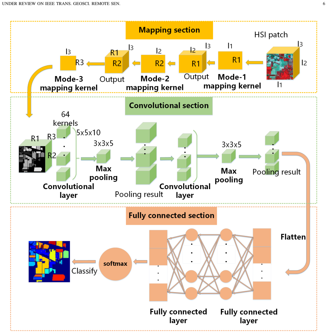
The load-bearing object is the mapping layer: each layer multiplies the input tensor along one mode by a factor matrix $U^{(n)}\in\mathbb{R}^{I_n\times R_n}$ obtained by solving the Tucker decomposition problem for the average training patch with alternating least squares and SVD. Three such layers, one per mode, reduce the spatial and spectral dimensions to $R_1$, $R_2$, $R_3$ and output a small energy-concentrated tensor. Because these kernels are fixed and not updated by back-propagation, the mapping section costs almost no training time, and the small 7x7x40 cube lets two 3-D convolutional layers do the feature extraction that deeper networks need many layers to achieve.
What would settle it
Take a hyperspectral dataset whose classes occupy noticeably different spectral subspaces, build the mapping kernels once from the global average patch and once from per-class average patches, and compare per-class accuracies; if the per-class kernels clearly outperform the global one, the single-average assumption is what limits the method.
Extended reading notes
Core claim
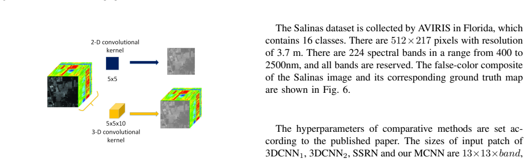
The central claim is that a neural network for hyperspectral image classification does not need many trainable layers if the input patch is first projected by fixed multilinear mapping kernels. The kernels are the three factor matrices from a Tucker decomposition of the single tensor obtained by averaging all training patches, and they reduce each 13x13x200 patch to a 7x7x40 cube, concentrating most of the energy while preserving the cube structure. A small 3-D convolutional section then extracts spectral-spatial features, and two fully connected layers classify them. The paper reports that this MCNN achieves the highest overall accuracy among the compared methods on all three benchmark datasets and that its total training time is substantially lower than that of the deep residual and deformable baselines.
Load-bearing premise
The whole method rests on the assumption that one tensor formed by averaging all training patches captures the common low-dimensional subspace of every patch well enough that the fixed projection keeps class-discriminative information while removing redundancy.
Editorial extensions
If this is right
- Classification accuracy on the three tested datasets rises to 98.3%, 99.5%, and 99.3%, all above the compared deep baselines.
- Total training time drops to tens of seconds on Indian Pines and Salinas, roughly an order of magnitude faster than the residual and deformable baselines.
- Replacing the mapping layers with PCA or per-patch tensor decomposition lowers accuracy and increases preprocessing time, indicating the averaged-patch projection is the source of the gain.
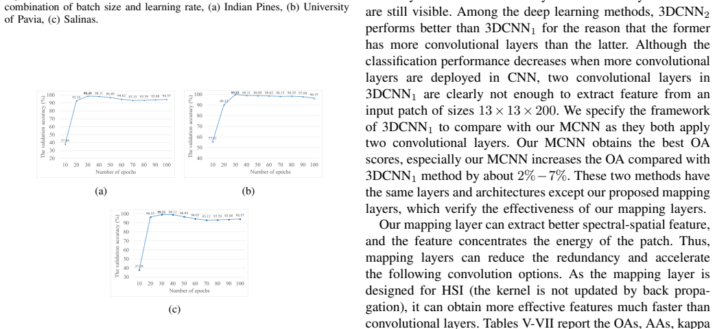
- A network with only two convolutional layers avoids the accuracy degradation that the paper associates with deeper hyperspectral CNNs.
Reading between the lines
- The same fixed mapping-layer design could be transferred to other tensor-structured inputs, such as video cubes or medical volume data, where a single average tensor may define a shared subspace for all samples.
- A natural stress test is to replace the single global average patch with class-wise average patches; if per-class kernels improve accuracy on datasets with spectrally distinct classes, the global averaging assumption is the limiting factor.
- Because the mapping kernels are computed once, one could update them incrementally as new labeled samples arrive, turning the architecture into a cheap few-shot or active-learning classifier.
- Combining the mapping layers with residual connections may address the gradient-vanishing limitation the paper itself notes, potentially allowing deeper convolutional sections without losing accuracy.
Signed reviews
Editorial analysis
A structured set of objections, weighed in public.
Referee Report
Summary. The manuscript proposes MCNN, a hyperspectral image classifier in which three fixed 'mapping layers' are constructed by a higher-order Tucker decomposition (ALS/HOOI) of the average training patch, reducing each 13×13×B input to 7×7×40 before two 3-D convolutional layers and two fully connected layers. The mapping weights are non-trainable, which the authors argue saves training time and avoids accuracy degradation with depth. On Indian Pines, University of Pavia, and Salinas, the method is reported to achieve the highest overall accuracy among SVM, EPF, two 3DCNNs, DHCNet, and SSRN (98.3%, 99.5%, 99.3%) with large reductions in total training time. The paper includes an ablation on Indian Pines comparing the mapping layers with PCA, raw data, and per-patch Tucker decomposition, plus runtime tables.
Significance. If the headline accuracy claim survives a leakage-free evaluation, the paper's contribution is a simple and inexpensive preprocessing module: fixed multilinear projections from a single averaged training patch, combined with a compact 3-D CNN, would be a practically useful baseline for HSI classification. The paper has strengths: three standard datasets; comparisons against six methods including two recent deep networks; multiple-run statistics with standard deviations; an ablation isolating the mapping-layer component; and a time comparison. The main weakness is that the experimental protocol does not exclude spatial overlap between training and test patches, so the central accuracy claim is not yet established.
major comments (3)
- [IV-A (data split) and III-A/Algorithm 1] The random 20/10/70 split of 13×13 patches is performed on patch indices, not on disjoint pixels. Neighboring patches overlap by up to 12 of 13 pixels in each spatial direction, so a large fraction of test patch content is present in the training set. Because the mapping kernels are computed from the average of all training patches (Algorithm 1, line 2), the unsupervised projection itself can absorb spatial/spectral information that overlaps the test set. This inflates the reported OA for all patch-based methods and may preferentially inflate MCNN. The margins over SSRN are small (IP: 98.3 vs 97.4; UP: 99.5 vs 99.3), so the claimed supremacy is not established. Please report results on spatially disjoint train/test splits (e.g., disjoint image blocks or a buffer zone between train and test regions), and quantify the overlap of the current split or justify why it does not bias the comparison.
- [IV-D and IV-C] The PCA protocol is ambiguous and, as written, unfair. In Section IV-D the authors state that 'PCA is employed as a preprocessing method on training dataset and testing dataset separately'; fitting PCA on the test set separately leaks test-set statistics into the features. If this procedure was also used for the 3DCNN1/3DCNN2/SSRN baselines in Tables V–VII, their accuracies are not comparable to MCNN. The comparison must fit PCA on the training split only and apply the same transformation to validation/test splits; the exact number of components, data centering, and whether PCA is applied per-patch or to the full image should be stated.
- [III-B and Fig. 2] The architecture description is internally inconsistent. For Indian Pines, the input to the first convolutional layer is 7×7×40 and the kernel is 5×5×10 with stride (1,1,5). Without padding this produces a 3×3×7×64 output, not the stated 5×5×54×64; padding, dilation, and channel layout are not specified. Since the comparison with 3DCNN1 is justified by 'the same layers and architectures except mapping layers', this discrepancy must be resolved with an exact layer-by-layer configuration.
minor comments (6)
- [IV-C] The claim that MCNN 'increases the OA compared with 3DCNN1 method by about 2%−7%' is inconsistent with Tables V–VII: the differences are 9.4, 2.0, and 4.4 percentage points on IP, UP, and Salinas, respectively.
- [Algorithm 1 and Section III-A] Use a distinct symbol (e.g., \bar{X}) for the averaged training patch; currently X denotes both the training patch tensor and its average, which is confusing.
- [Equation (4)] Equation (4) contains an index error: after the mode-n product the mode-n index should be the column index of U, and the summation should run over the original mode-n index. Please correct.
- [End of Section IV-D] The sentence 'The disadvantage of our MCNN is that it only avoids the gradient vanishing problem, this problem can only be sovled by residual network so far' is unclear and contains a typo; please state precisely what limitation is intended (e.g., the fixed mapping layers are not learned and may not adapt to heterogeneous patches).
- [Section III-A and Section V] The claim that 'most energy of the input is preserved' is never quantified. Report the retained Tucker energy (e.g., sum of retained core entries divided by total energy) for the chosen (R1,R2,R3) on each dataset, or soften the claim.
- [Tables VIII-X] The DHCNet rows list no per-epoch time or epoch count, so the total training time cannot be interpreted; specify the protocol used to obtain these numbers.
Circularity Check
No significant circularity: the mapping layers are unsupervised projections and the reported accuracies are measured on held-out pixels.
full rationale
The paper's derivation chain is self-contained and empirical: the mapping kernels U^(1), U^(2), U^(3) are obtained by a Tucker decomposition of the averaged training patch (Algorithm 1, Section III-A), using only unlabeled tensor structure, not class labels. The classification accuracies reported in Tables V–VII are measured on a held-out test split after training the CNN with backpropagation, so no test quantity is used to construct the mapping layers, and no fitted parameter is renamed as a prediction. The claim that the mapping layers preserve most of the input energy follows from the well-known optimality of singular vectors for low-rank reconstruction; the paper does not quantify it, which is an unsubstantiated assertion rather than a circular reduction. Comparisons against SSRN, DHCNet, 3DCNN, EPF, and SVM are standard external benchmark comparisons, and the paper's self-citations are ordinary references to prior methods, not load-bearing uniqueness arguments. The potential concern that randomly split overlapping patches may cause spatial leakage is an experimental-validity issue, not a circularity of the argument, because the reported numbers are measurements rather than consequences of the mapping-layer construction by definition. No equation in the paper reduces to its own inputs, and no specific circular step could be exhibited.
Assumptions & free parameters
free parameters (5)
- R1, R2, R3 (mapping layer output sizes) =
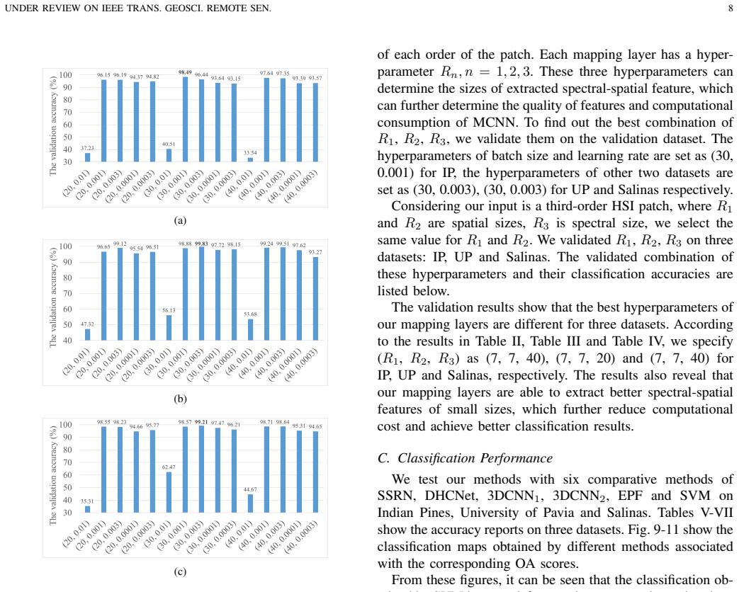
(7,7,40) for Indian Pines and Salinas; (7,7,20) for University of Pavia
- Learning rate =
0.001 for Indian Pines; 0.003 for University of Pavia and Salinas
- Batch size =
30 for all datasets
- Training epochs =
30 for all datasets
- ALS stopping threshold =
0.01 on difference of core tensors
assumptions (4)
- domain assumption Tucker decomposition of the average training patch identifies a subspace that is representative of all training patches.
- domain assumption The energy concentration property of truncated singular vectors guarantees that the mapping keeps the most discriminative information for classification.
- domain assumption Random pixel-level patch splitting gives a valid estimate of generalization.
- standard math Standard multilinear algebra operations (mode-n product, SVD) behave as described.
Cite this review
Pith. "Pith review of A Convolutional Neural Network with Mapping Layers for Hyperspectral Image Classification." pith.science (2026). https://pith.science/paper/QYOWCZBG
@misc{pith2026190809526,
  author       = {Pith},
  title        = {Pith review of: A Convolutional Neural Network with Mapping Layers for Hyperspectral Image Classification},
  year         = {2026},
  howpublished = {\url{https://pith.science/paper/QYOWCZBG}},
  note         = {Machine review of arXiv:1908.09526}
}
read the original abstract
In this paper, we propose a convolutional neural network with mapping layers (MCNN) for hyperspectral image (HSI) classification. The proposed mapping layers map the input patch into a low dimensional subspace by multilinear algebra. We use our mapping layers to reduce the spectral and spatial redundancy and maintain most energy of the input. The feature extracted by our mapping layers can also reduce the number of following convolutional layers for feature extraction. Our MCNN architecture avoids the declining accuracy with increasing layers phenomenon of deep learning models for HSI classification and also saves the training time for its effective mapping layers. Furthermore, we impose the 3-D convolutional kernel on convolutional layer to extract the spectral-spatial features for HSI. We tested our MCNN on three datasets of Indian Pines, University of Pavia and Salinas, and we achieved the classification accuracy of 98.3%, 99.5% and 99.3%, respectively. Experimental results demonstrate that the proposed MCNN can significantly improve the classification accuracy and save much time consumption.
Figures

Figures from the paper (6 more)



Reference graph
Works this paper leans on
-
[1]
Modern trends in hyperspectral image analysis: A review,
M. J. Khan, H. S. Khan, A. Yousaf, K. Khurshid, and A. Abbas, “Modern trends in hyperspectral image analysis: A review,” IEEE Access, vol. 6, pp. 14 118–14 129, Mar. 2018
2018
-
[2]
Semi-supervised learning through label propagation on geodesics,
M. Fan, X. Zhang, L. Du, L. Chen, and D. Tao, “Semi-supervised learning through label propagation on geodesics,” IEEE Trans. Cybern., vol. 48, no. 5, pp. 1486–1499, Jul. 2018
work page 2018
-
[3]
Extended random walker-based classification of hyperspectral images,
X. Kang, S. Li, L. Fang, M. Li, and J. A. Benediktsson, “Extended random walker-based classification of hyperspectral images,” IEEE Trans. Geosci. Remote Sens. , vol. 53, no. 1, pp. 144–153, Dec. 2015
work page 2015
-
[4]
Salient band selection for hyperspectral image classification via manifold ranking,
Q. Wang, J. Lin, and Y . Yuan, “Salient band selection for hyperspectral image classification via manifold ranking,” IEEE Trans. Neural Netw. Learn. Syst., vol. 27, no. 6, pp. 1279–1289, Jun. 2016
work page 2016
-
[5]
Similarity-based unsupervised band selection for hyperspectral image analysis
Q. Du and H. Yang, “Similarity-based unsupervised band selection for hyperspectral image analysis.” IEEE Geosci. Remote Sens. Lett. , vol. 5, no. 4, pp. 564–568, Oct. 2008
work page 2008
-
[6]
Y . Yuan, J. Lin, and Q. Wang, “Hyperspectral image classification via multitask joint sparse representation and stepwise mrf optimization,” IEEE Trans. Cybern. , vol. 46, no. 12, pp. 2966–2977, Dec. 2016
work page 2016
-
[7]
J. Jiang, J. Ma, C. Chen, Z. Wang, Z. Cai, and L. Wang, “Superpca: A superpixelwise pca approach for unsupervised feature extraction of hyperspectral imagery,” IEEE Trans. Geosci. Remote Sens. , vol. 56, no. 8, pp. 4581–4593, Aug. 2018
work page 2018
-
[8]
Limitations of principal components analysis for hyperspectral target recognition,
S. Prasad and L. M. Bruce, “Limitations of principal components analysis for hyperspectral target recognition,” IEEE Geosci. Remote Sens. Lett., vol. 5, no. 4, pp. 625–629, Oct. 2008
work page 2008
Show all 41 references
-
[9]
Unsupervised feature ex- traction based on a mutual information measure for hyperspectral image classification,
M. A. Hossain, M. Pickering, and X. Jia, “Unsupervised feature ex- traction based on a mutual information measure for hyperspectral image classification,” in Proc. IEEE Int. Geosci. Remote Sens. Symp. (IGARSS), 2011, pp. 1720–1723
2011
-
[10]
Dimensionality reduction via regression in hyperspectral imagery,
V . Laparra, J. Malo, and G. Camps-Valls, “Dimensionality reduction via regression in hyperspectral imagery,” IEEE J. Sel. Topics Signal Process., vol. 9, no. 6, pp. 1026–1036, Sep. 2015
2015
-
[11]
Classification of hyperspectral images with regularized linear discriminant analysis,
T. V . Bandos, L. Bruzzone, and G. Camps-Valls, “Classification of hyperspectral images with regularized linear discriminant analysis,” IEEE Trans. Geosci. Remote Sens. , vol. 47, no. 3, pp. 862–873, Mar. 2009
2009
-
[12]
A modified locality-preserving projection approach for hyperspectral image classification,
Y . Zhai, L. Zhang, N. Wang, Y . Guo, Y . Cen, T. Wu, and Q. Tong, “A modified locality-preserving projection approach for hyperspectral image classification,” IEEE Geosci. Remote Sens. Lett. , vol. 13, no. 8, pp. 1059–1063, Aug. 2016
2016
-
[13]
Discover latent discriminant information for dimensional- ity reduction: Non-negative sparseness preserving embedding,
W. K. Wong, “Discover latent discriminant information for dimensional- ity reduction: Non-negative sparseness preserving embedding,” Pattern recognition, vol. 45, no. 4, pp. 1511–1523, Apr. 2012
2012
-
[14]
Locality and structure regularized low rank representation for hyperspectral image classification,
Q. Wang, X. He, and X. Li, “Locality and structure regularized low rank representation for hyperspectral image classification,” IEEE Trans. Geosci. Remote Sens. , vol. 57, no. 2, pp. 911–923, Feb. 2018
2018
-
[15]
Spectral–spatial hyperspectral image classification with edge-preserving filtering,
X. Kang, S. Li, and J. A. Benediktsson, “Spectral–spatial hyperspectral image classification with edge-preserving filtering,” IEEE Trans. Geosci. Remote Sens., vol. 52, no. 5, pp. 2666–2677, May 2014
2014
-
[16]
Kernel-based methods for hyperspec- tral image classification,
G. Camps-Valls and L. Bruzzone, “Kernel-based methods for hyperspec- tral image classification,” IEEE Trans. Geosci. Remote Sens. , vol. 43, no. 6, pp. 1351–1362, Jun. 2005
2005
-
[17]
Classification and feature extraction for remote sensing images from urban areas based on morphological transformations,
J. A. Benediktsson, M. Pesaresi, and K. Amason, “Classification and feature extraction for remote sensing images from urban areas based on morphological transformations,” IEEE Trans. Geosci. Remote Sens. , vol. 41, no. 9, pp. 1940–1949, Sep. 2003
1940
-
[18]
Composite kernels for hyperspectral image classification,
G. Camps-Valls, L. Gomez-Chova, J. Mu ˜noz-Mar´ı, J. Vila-Franc ´es, and J. Calpe-Maravilla, “Composite kernels for hyperspectral image classification,” IEEE Geosci. Remote Sens. Lett., vol. 3, no. 1, pp. 93–97, Jan. 2006
2006
-
[19]
Video segmentation with superpixels,
F. Galasso, R. Cipolla, and B. Schiele, “Video segmentation with superpixels,” in Proc. ACCV. Springer, 2012, pp. 760–774
2012
-
[20]
Representation learning: A review and new perspectives,
Y . Bengio, A. Courville, and P. Vincent, “Representation learning: A review and new perspectives,” IEEE Trans. Pattern Anal. Mach. Intell. , vol. 35, no. 8, pp. 1798–1828, Aug. 2013
2013
-
[21]
Deep hierarchies in the primate visual cortex: What can we learn for computer vision?
N. Kruger, P. Janssen, S. Kalkan, M. Lappe, A. Leonardis, J. Piater, A. J. Rodriguez-Sanchez, and L. Wiskott, “Deep hierarchies in the primate visual cortex: What can we learn for computer vision?” IEEE Trans. Pattern Anal. Mach. Intell. , vol. 35, no. 8, pp. 1847–1871, Aug. 2013
2013
-
[22]
Deep learning-based classification of hyperspectral data,
Y . Chen, Z. Lin, X. Zhao, G. Wang, and Y . Gu, “Deep learning-based classification of hyperspectral data,” IEEE J. Sel. Topics Appl. Earth Observ. Remote Sens. , vol. 7, no. 6, pp. 2094–2107, Jun. 2014
2014
-
[23]
Spectral–spatial feature extraction for hsi classification based on supervised hypergraph and sample expanded cnn,
Y . Kong, X. Wang, and Y . Cheng, “Spectral–spatial feature extraction for hsi classification based on supervised hypergraph and sample expanded cnn,” IEEE J. Sel. Topics Appl. Earth Observ. Remote Sens. , vol. 11, no. 11, pp. 4128–4140, Nov. 2018
2018
-
[24]
Cnn-based multilayer spatial–spectral feature fusion and sample aug- mentation with local and nonlocal constraints for hyperspectral image classification,
J. Feng, J. Chen, L. Liu, X. Cao, X. Zhang, L. Jiao, and T. Yu, “Cnn-based multilayer spatial–spectral feature fusion and sample aug- mentation with local and nonlocal constraints for hyperspectral image classification,” IEEE J. Sel. Topics Appl. Earth Observ. Remote Sens. , vo...
2019
-
[25]
Multisource remote sensing data classification based on convolutional neural network,
X. Xu, W. Li, Q. Ran, Q. Du, L. Gao, and B. Zhang, “Multisource remote sensing data classification based on convolutional neural network,” IEEE Trans. Geosci. Remote Sens. , vol. 56, no. 2, pp. 937–949, Feb. 2017
2017
-
[26]
Scene classification with recurrent attention of vhr remote sensing images,
Q. Wang, S. Liu, J. Chanussot, and X. Li, “Scene classification with recurrent attention of vhr remote sensing images,” IEEE Trans. Geosci. Remote Sens., vol. 57, no. 2, pp. 1156–1167, Feb. 2019
2019
-
[27]
Deep feature extraction and classification of hyperspectral images based on convolutional neural networks,
Y . Chen, H. Jiang, C. Li, X. Jia, and P. Ghamisi, “Deep feature extraction and classification of hyperspectral images based on convolutional neural networks,” IEEE Trans. Geosci. Remote Sens., vol. 54, no. 10, pp. 6232– 6251, Oct. 2016
2016
-
[28]
Stacked denoising autoencoders: Learning useful representations in a deep network with a local denoising criterion,
P. Vincent, H. Larochelle, I. Lajoie, Y . Bengio, and P.-A. Manzagol, “Stacked denoising autoencoders: Learning useful representations in a deep network with a local denoising criterion,” J. Mach. Learn. Res. , vol. 11, no. Dec, pp. 3371–3408, Dec. 2010
2010
-
[29]
Convolutional deep belief networks for scalable unsupervised learning of hierarchical representations,
H. Lee, R. Grosse, R. Ranganath, and A. Y . Ng, “Convolutional deep belief networks for scalable unsupervised learning of hierarchical representations,” in Proc. Int’l Conf. Mach. Learn. ACM, 2009, pp. 609–616
2009
-
[30]
Going deeper with contextual cnn for hyperspec- tral image classification,
H. Lee and H. Kwon, “Going deeper with contextual cnn for hyperspec- tral image classification,” IEEE Trans. Image Process. , vol. 26, no. 10, pp. 4843–4855, Oct. 2017
2017
-
[31]
Spectral-spatial residual network for hyperspectral image classification: A 3-d deep learning framework,
Z. Zhong, J. Li, Z. Luo, and M. Chapman, “Spectral-spatial residual network for hyperspectral image classification: A 3-d deep learning framework,” IEEE Trans. Geosci. Remote Sens., vol. 56, no. 2, pp. 847– 858, Feb. 2018
2018
-
[32]
High-order possibilistic c- means algorithms based on tensor decompositions for big data in iot,
Q. Zhang, L. T. Yang, Z. Chen, and P. Li, “High-order possibilistic c- means algorithms based on tensor decompositions for big data in iot,” Inf. Fusion, vol. 39, pp. 72–80, Jan. 2018
2018
-
[33]
Foundations of the parafac procedure: Models and conditions for an
R. A. Harshman, “Foundations of the parafac procedure: Models and conditions for an” explanatory” multimodal factor analysis,” UCLA Working Papers in Phonetics, Dec. 1970
1970
-
[34]
A multilinear singular value decomposition,
L. De Lathauwer, B. De Moor, and J. Vandewalle, “A multilinear singular value decomposition,” SIAM J. Matrix Anal. Appl. , vol. 21, no. 4, pp. 1253–1278, Apr. 2000
2000
-
[35]
Some mathematical notes on three-mode factor analysis,
L. R. Tucker, “Some mathematical notes on three-mode factor analysis,” Psychometrika, vol. 31, no. 3, pp. 279–311, 1966
1966
-
[36]
Very deep convolutional networks for large-scale image recognition,
K. Simonyan and A. Zisserman, “Very deep convolutional networks for large-scale image recognition,” arXiv preprint arXiv:1409.1556 , 2014. UNDER REVIEW ON IEEE TRANS. GEOSCI. REMOTE SEN. 13
2014 arXiv
-
[37]
Deep learning,
Y . LeCun, Y . Bengio, and G. Hinton, “Deep learning,”Nature, vol. 521, no. 7553, p. 436, Sep. 2015
2015
-
[38]
Human-level control through deep reinforcement learning,
V . Mnih, K. Kavukcuoglu, D. Silver, A. A. Rusu, J. Veness, M. G. Bellemare, A. Graves, M. Riedmiller, A. K. Fidjeland, G. Ostrovski et al. , “Human-level control through deep reinforcement learning,” Nature, vol. 518, no. 7540, pp. 529–533, Feb. 2015
2015
-
[39]
Deformable convolutional neural networks for hyperspectral image classification,
J. Zhu, L. Fang, and P. Ghamisi, “Deformable convolutional neural networks for hyperspectral image classification,” IEEE Geosci. Remote Sens. Lett., vol. 15, no. 8, pp. 1254–1258, Aug. 2018
2018
-
[40]
Spectral–spatial classification of hyper- spectral imagery with 3d convolutional neural network,
Y . Li, H. Zhang, and Q. Shen, “Spectral–spatial classification of hyper- spectral imagery with 3d convolutional neural network,” Remote Sens., vol. 9, no. 1, p. 67, 2017
2017
-
[41]
Libsvm: a library for support vector machines,
C.-C. Chang and C.-J. Lin, “Libsvm: a library for support vector machines,” ACM TIST, vol. 2, no. 3, p. 27, Apr. 2011. Rui Li received the B. S. and M. S. degree from Xidian University, Xi’an, P. R. China, in 2012 and 2015 respectively. He is currently working towards the Ph. ...
2011
Reviewed August 14, 2026 · model on record in the stance chip above.
Discussion (0). Continue with ORCID to comment.